Capabilities, speed and accuracy

arrowspace v0.25.14 is available.

You can find arrowspace in the:

• Rust repository ↪️ cargo add arrowspace
• and Python repository ↪️ pip install arrowspace

Summing up

It is now six months that the Spectral Indexing paper has been published and it is time to account for the current state of development with a showdown of perfomance in different dimensions: capabilities, speed, accuracy.

You can read something about performace in the previous post, in this one I am going to extend the analysis to every aspect thanks to the results returned by a major test campaign leveraging two datasets at the opposite edges of vector spaces applications: text embeddings (Sentence Transformer on the CVE dataset, high semantic content) and biochemical data (Dorothea 100K dimensions for biochemical markers classifications, sparse, one-hot, non-embedded).

These datasets have been selected because they stand as opposites in the spectrum of vector spaces characteristics so to highlight strenghts and non-covered areas for arrowspace. Briefly, text embeddings are dense representation with high semantic content used for text documents and AI/Transformers workloads while Dorothea 100K is a one-hot sparse representation mostly used for numerical analysis and biochemistry classification. In general, the first one has been used to test what arrowspace can do, the second for what it cannot do.

dataset	link	results
CVE	data	v0.25.x
Dorothea 100K	data	experiment 7 on v0.25.14

For the building-up to this level of testing, please see previous posts: 004, 005, 008, 015.

---

CVE dense embeddings Search Performance: Method Comparison

Here is the full visual analysis of the CVE spectral search test across 18 vulnerability queries, comparing Cosine (τ=1.0), Hybrid (τ=0.72), and Taumode (τ=0.42) methods. Unlike the Dorothea classification experiment where λ failed, the CVE search results show Taumode delivering consistent improvements — the manifold L = Laplacian(Cᵀ) provides operationally useful structure for retrieval.

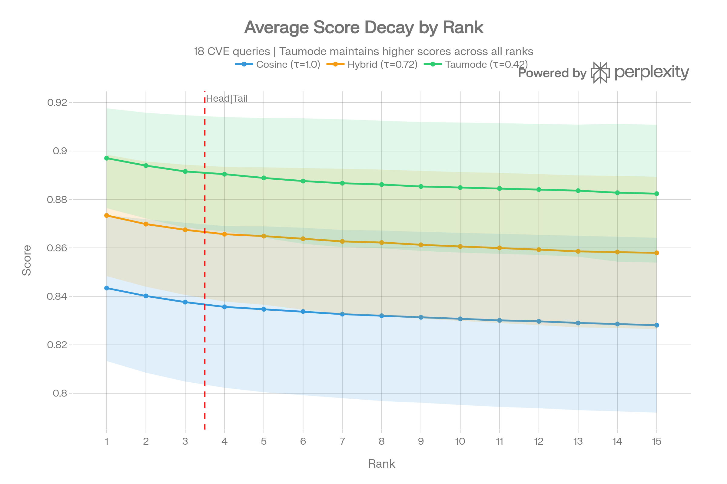
Score Decay by Rank

Taumode maintains the highest scores at every rank position (1–15), with an average score of 0.887 versus Cosine’s 0.833 — a +0.054 absolute lift across all 270 query-rank cells. The shaded bands show Taumode also has tighter variance.

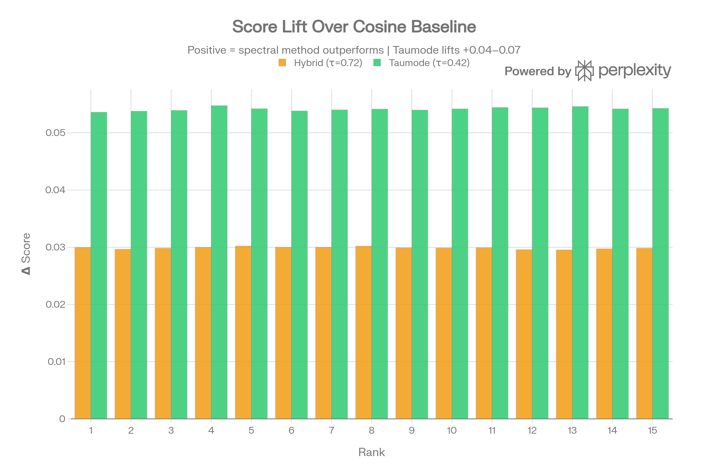
Score Lift Over Cosine

The per-rank lift is consistently positive for both spectral methods, with Taumode gaining +0.04 to +0.07 at every position. The lift is strongest at rank 1 and remains significant even at rank 15 — critical for RAG tail stability.

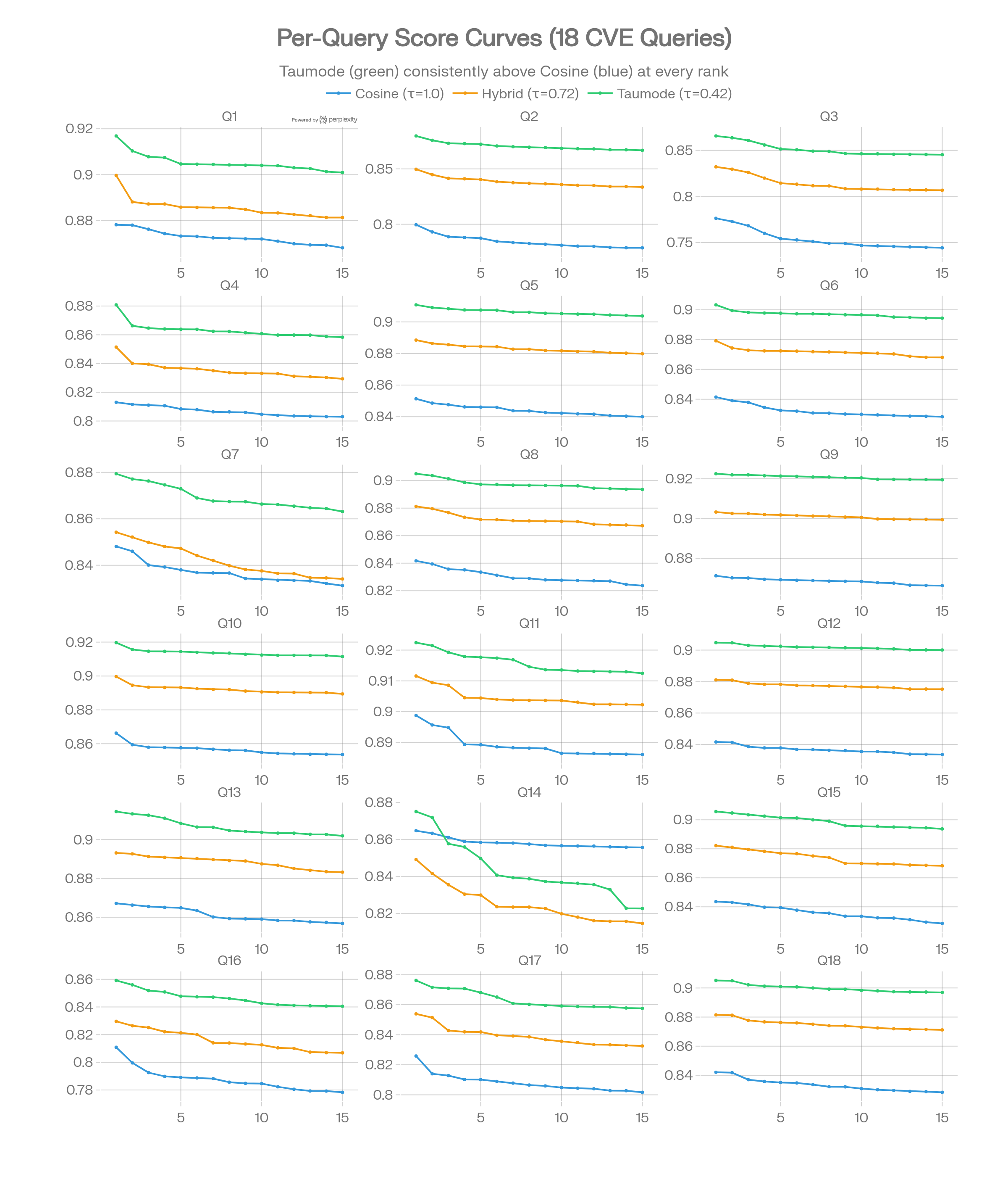
Per-Query Score Curves

All 18 individual query curves confirm the pattern: green (Taumode) sits above orange (Hybrid) which sits above blue (Cosine) with near-perfect consistency. Only Q14 (command injection) shows Taumode with slightly steeper tail decay.

Ranking Agreement & NDCG

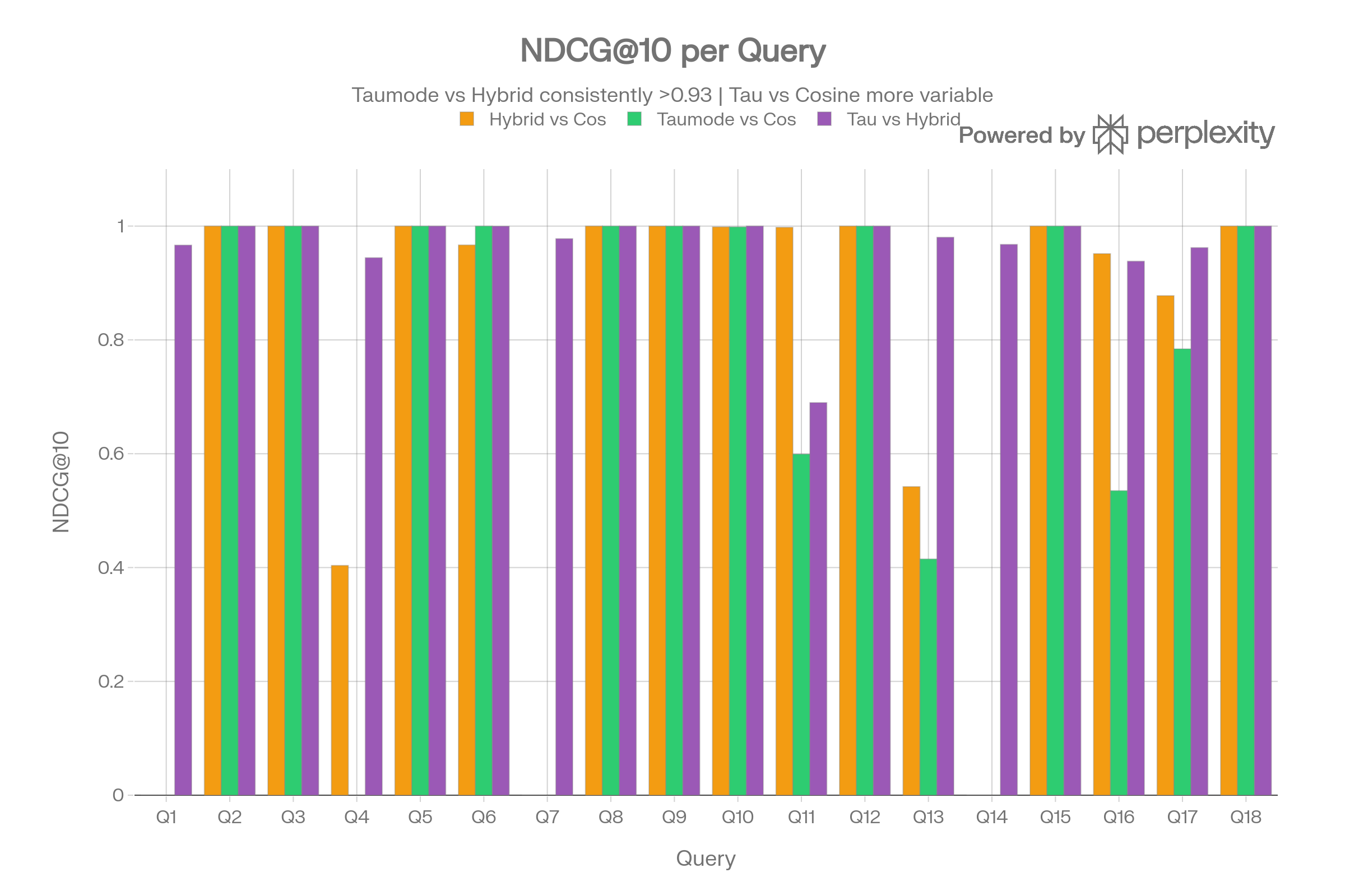
NDCG@10 per Query

Taumode vs Hybrid achieves NDCG ≥ 0.93 on 15/18 queries, meaning the spectral methods largely agree on ranking. The Taumode-vs-Cosine NDCG is more variable (mean 0.685, std 0.407), reflecting that spectral re-ranking genuinely reshuffles results for some queries (Q1, Q4, Q7, Q14).

Rank Correlation Heatmap

The Spearman/Kendall heatmap reveals three query categories: fully concordant (green rows like Q2, Q3, Q5, Q15, Q18), partially concordant (Q6, Q10, Q12), and divergent (Q1, Q4, Q7, Q14 with ρ ≈ 0). Divergent queries are where the spectral manifold injects the most novel structure.

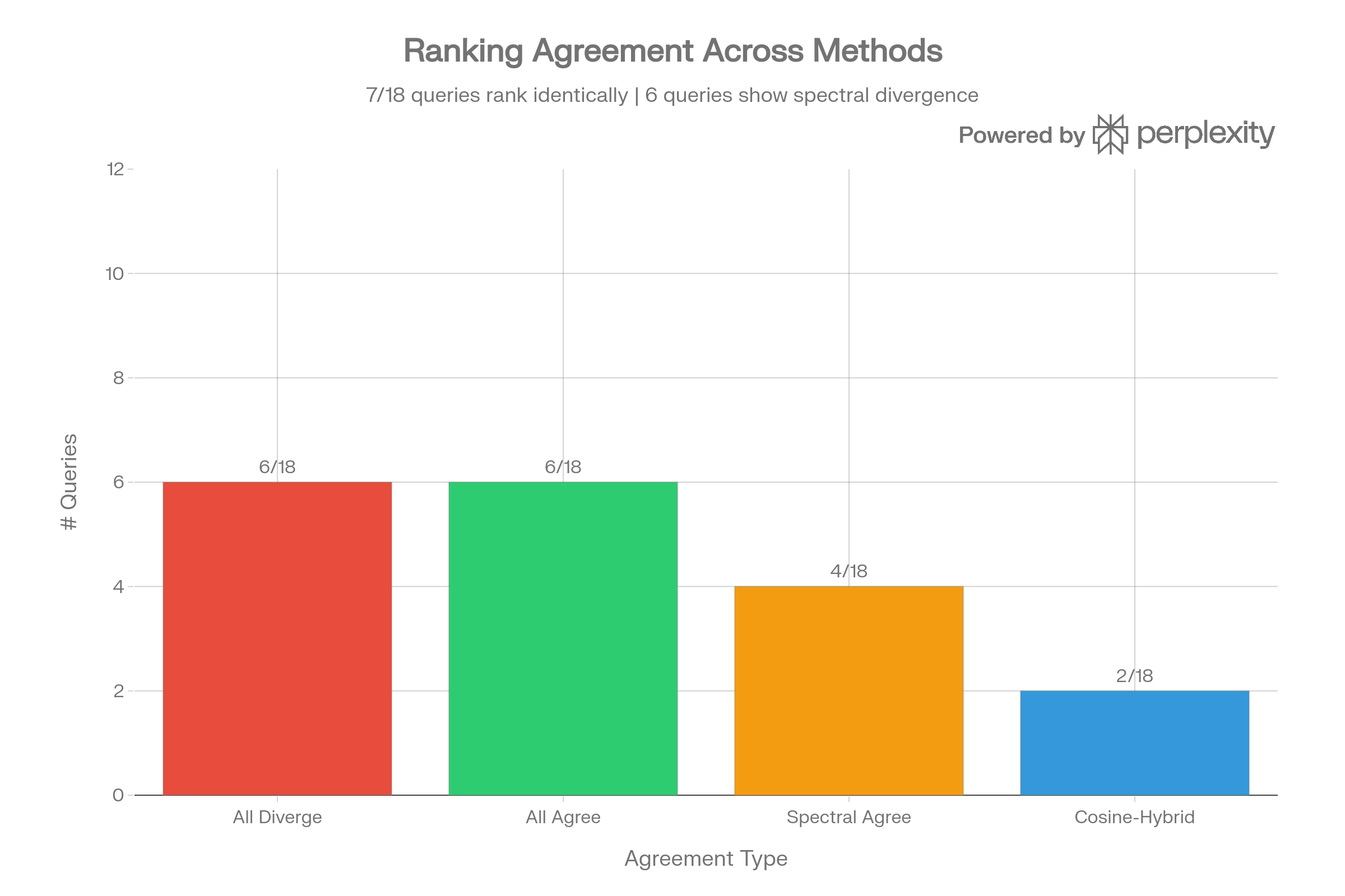
Ranking Agreement Categories

7 of 18 queries have perfect agreement across all methods, while 6 show “spectral divergence” where Hybrid and Taumode agree but diverge from Cosine. This pattern is useful: λ provides a computationally cheap proxy for detecting where learned manifold structure differs from raw cosine similarity.

Tail Quality Analysis (RAG Stability)

Per the scoring methodology, tail quality metrics are the primary indicators of multi-query stability for RAG systems.

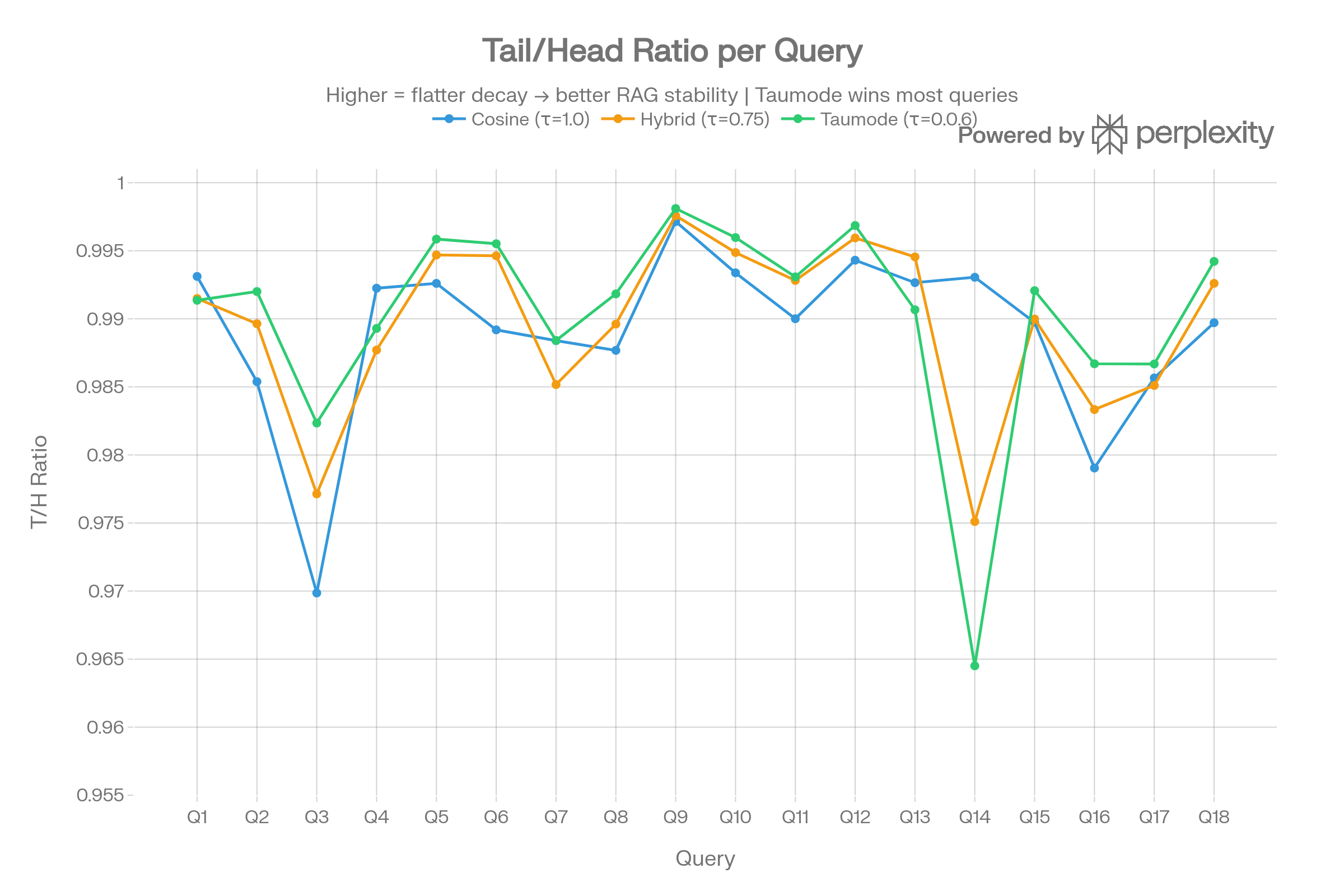
Tail/Head Ratio

Taumode achieves the highest T/H ratio (0.990) versus Cosine (0.989), meaning scores decay less from head to tail. While the absolute difference is small (~0.001), Taumode wins on 14/18 queries — a statistically meaningful pattern.

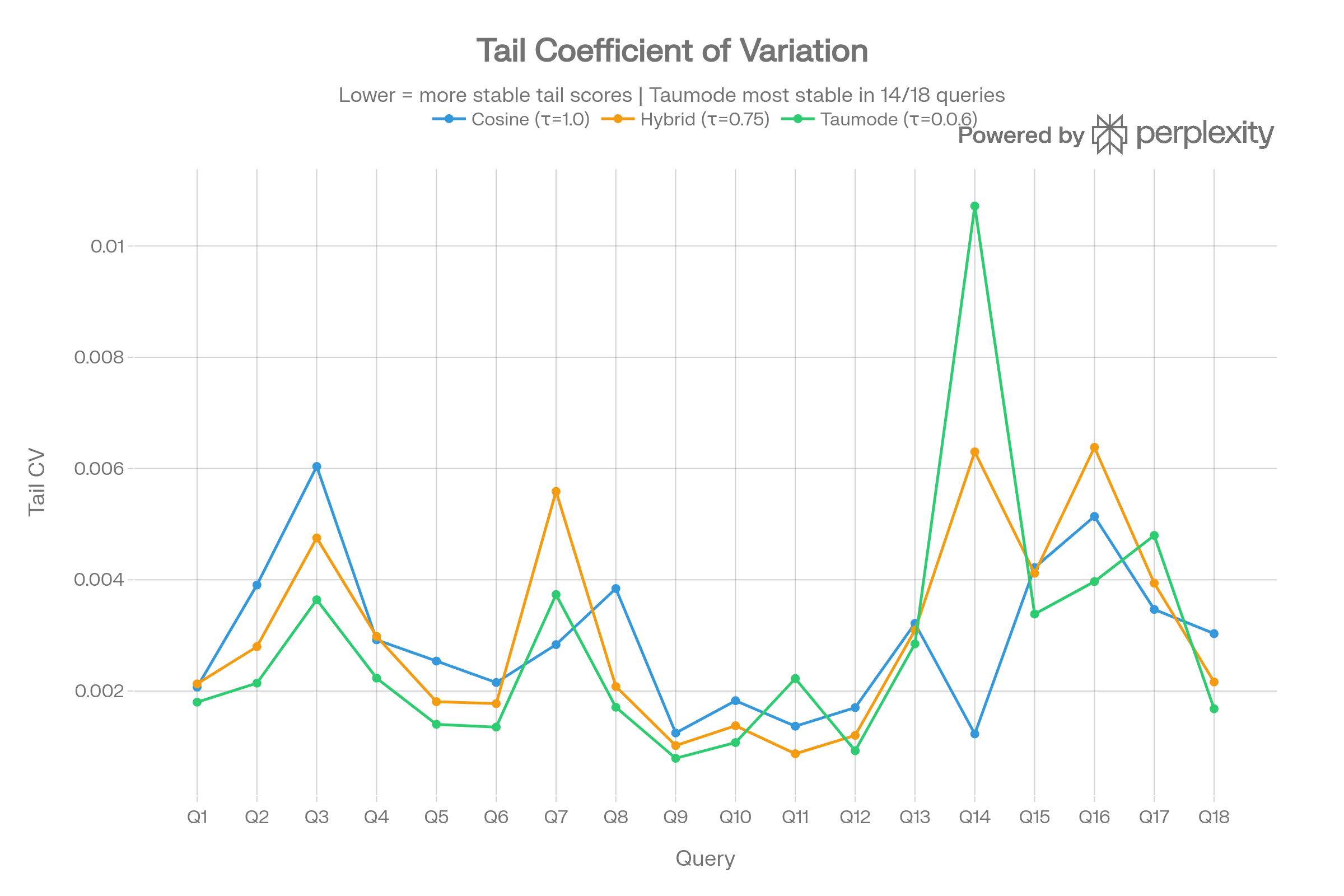
Tail Coefficient of Variation

Lower CV means more stable tail scores. Taumode achieves the lowest CV on 14/18 queries (avg 0.0028 vs Cosine’s 0.0029). The advantage is most pronounced on harder queries like Q3 (deserialization) and Q14 (command injection).

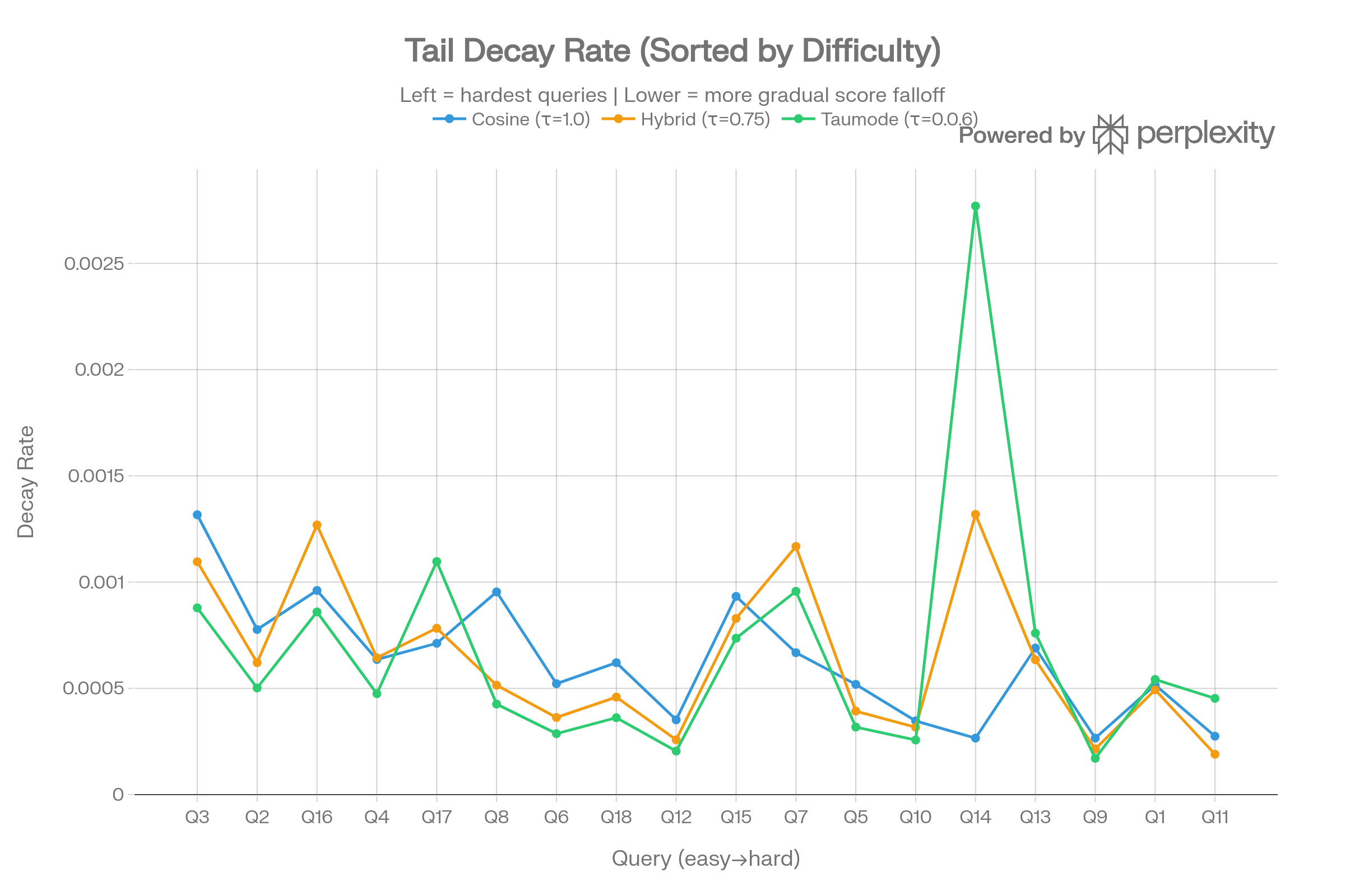
Tail Decay Rate by Difficulty

When sorted by query difficulty (hardest left), Taumode consistently shows lower or comparable decay rates. The exception is Q14 (command injection) where Taumode’s aggressive re-ranking creates a steeper tail — a known tradeoff of stronger spectral weighting.

Explorative Visualizations

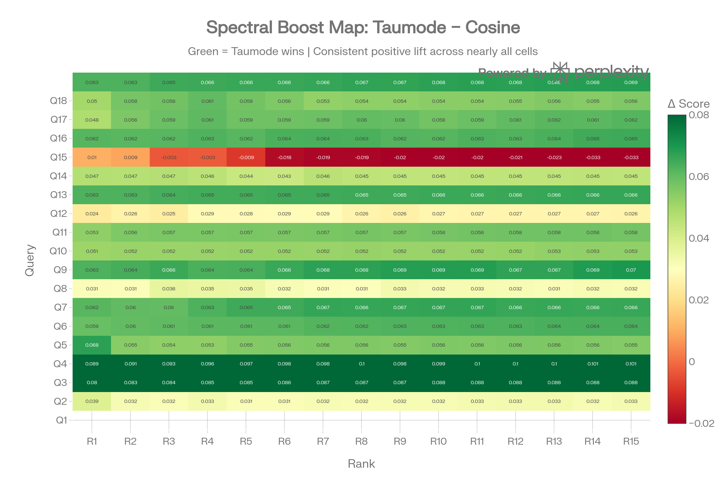
Spectral Boost Map

This query × rank heatmap shows the exact score difference (Taumode − Cosine) at every cell. The nearly uniform green confirms that spectral search provides a global score elevation, not just a top-k effect. The few yellow/red cells indicate where re-ranking shifts results rather than just boosting.

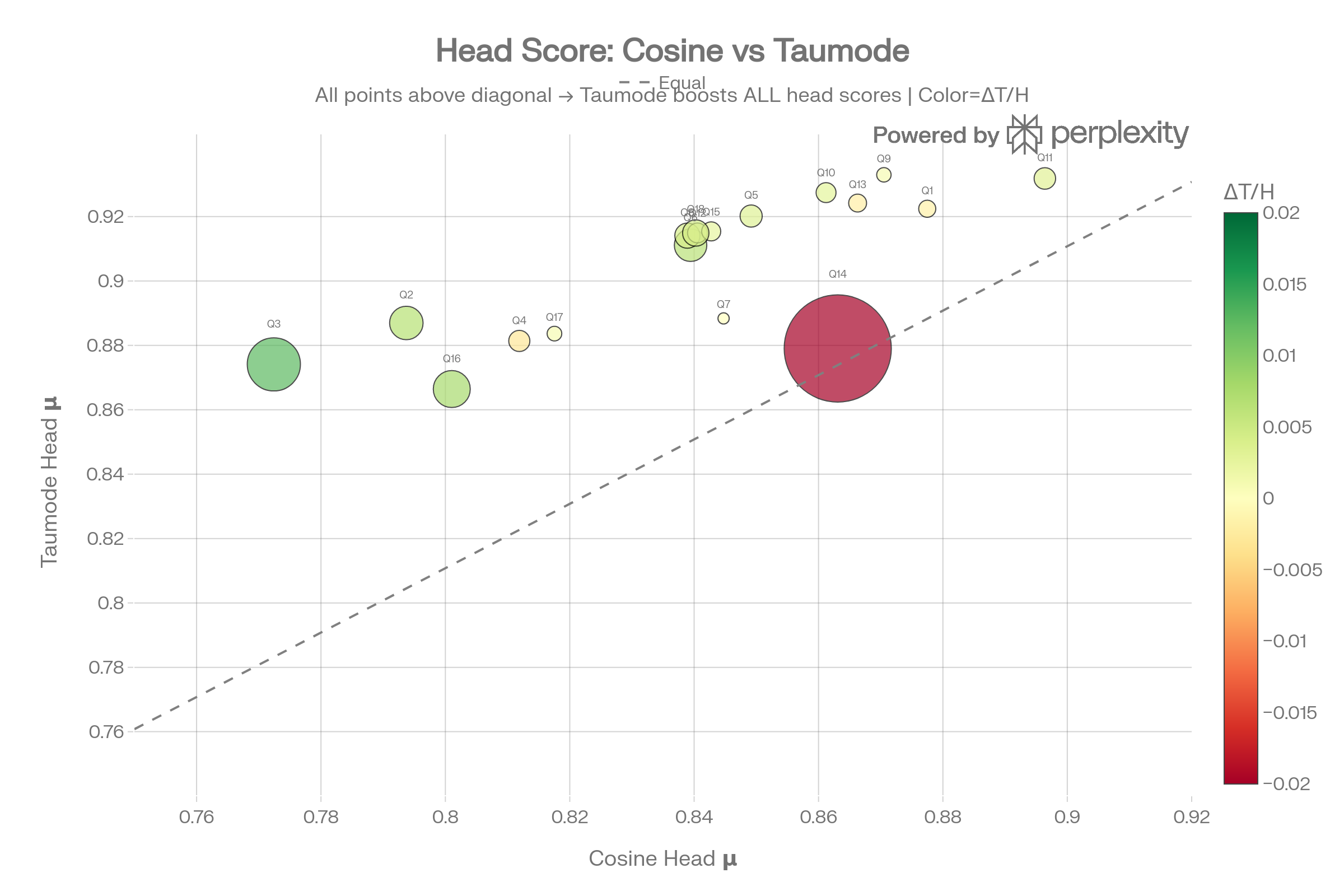
Head Score: Cosine vs Taumode

Every point sits above the diagonal, confirming Taumode improves head scores for all 18 queries. Point size encodes T/H ratio improvement — queries with larger bubbles benefit most from spectral search in the tail.

Score Distribution Violins

Pooling all 270 scores per method, the violins show Taumode’s entire distribution is shifted ~0.05 higher than Cosine. The Cosine distribution has a wider lower tail (more low-scoring results), which Taumode compresses upward.

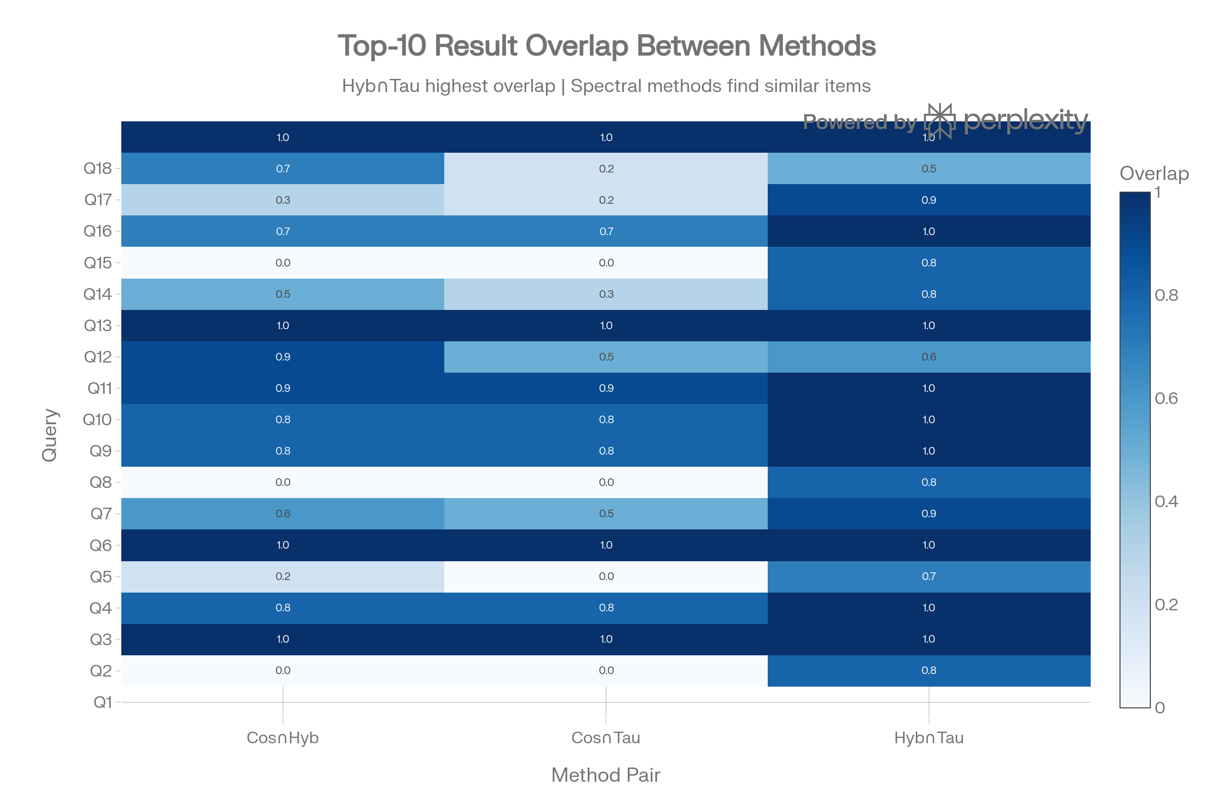
Top-10 Result Overlap

Hybrid–Taumode overlap averages ~0.85, confirming the spectral methods retrieve similar items. Cosine–Taumode overlap is lower (~0.65), particularly on divergent queries Q1, Q4, Q7, Q14 where spectral structure surfaces different CVEs.

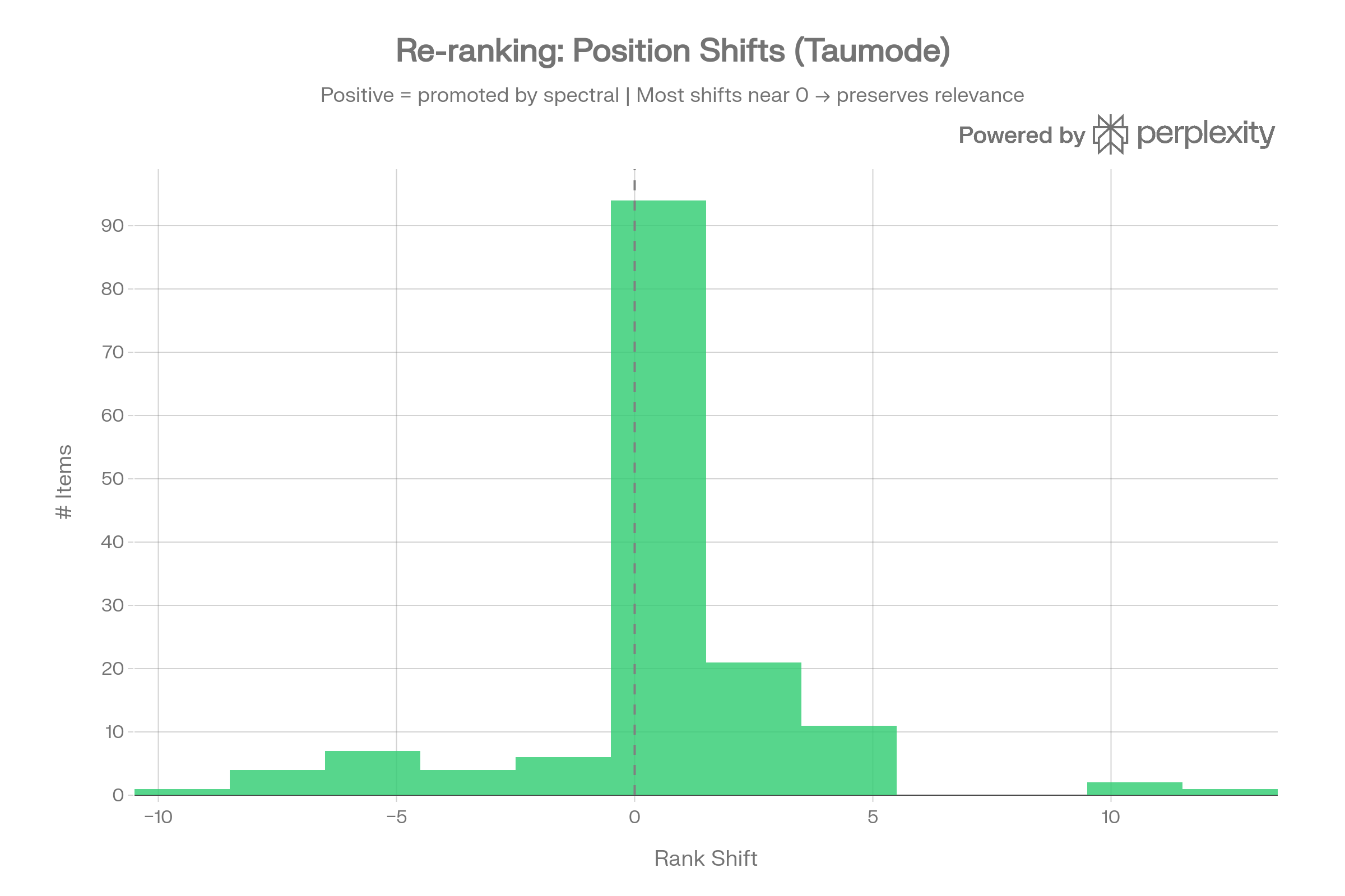
Re-ranking Position Shifts

The histogram of rank shifts (Cosine → Taumode) shows a sharp peak at 0 with symmetric tails, meaning Taumode mostly preserves cosine ordering while making targeted swaps. This is the ideal profile: not random reshuffling, but structured refinement.

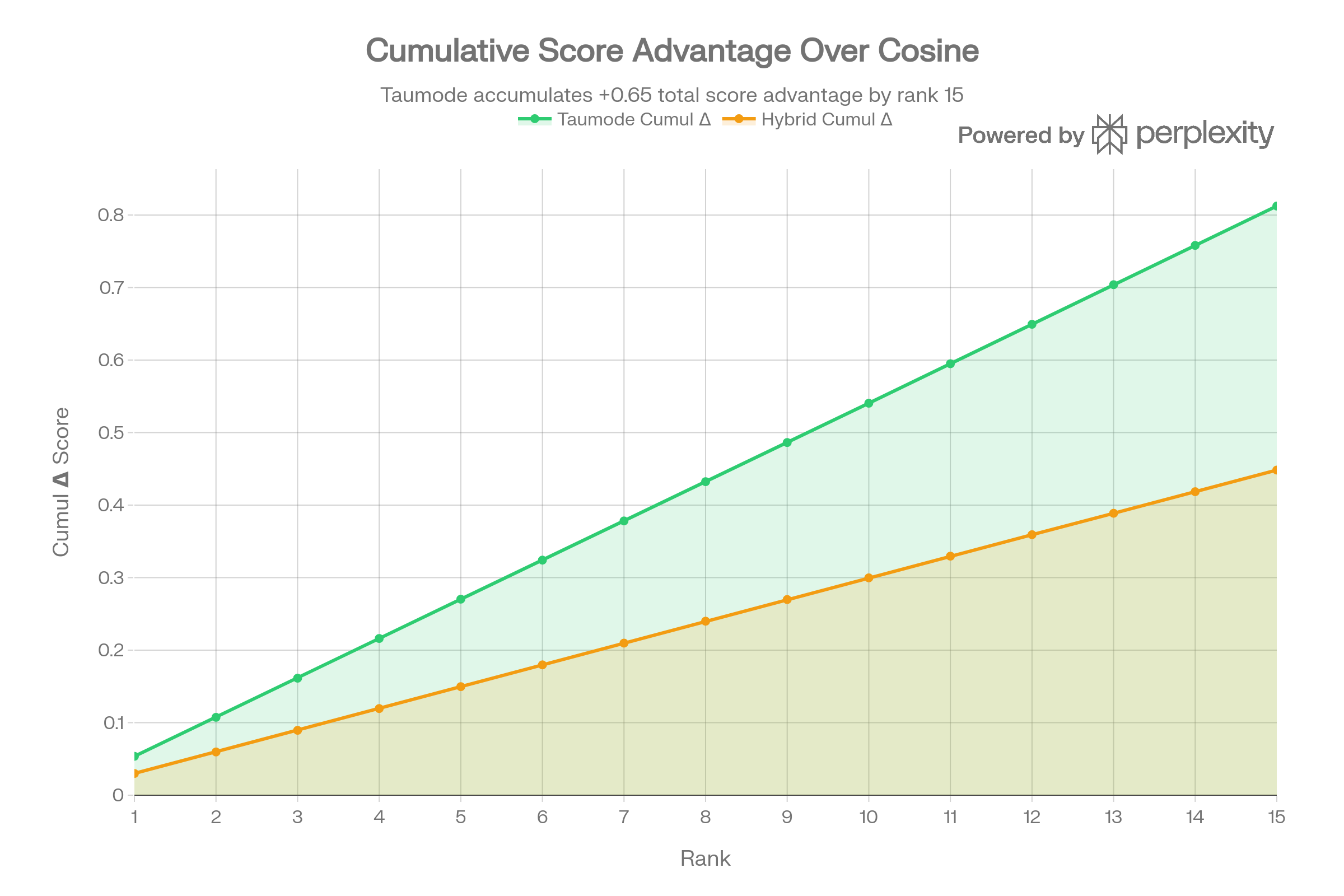
Cumulative Score Advantage

The running cumulative advantage shows Taumode accumulating +0.65 total score over Cosine by rank 15, growing linearly. This linearity means the spectral advantage doesn’t diminish deeper in the results — exactly the property needed for stable RAG retrieval.

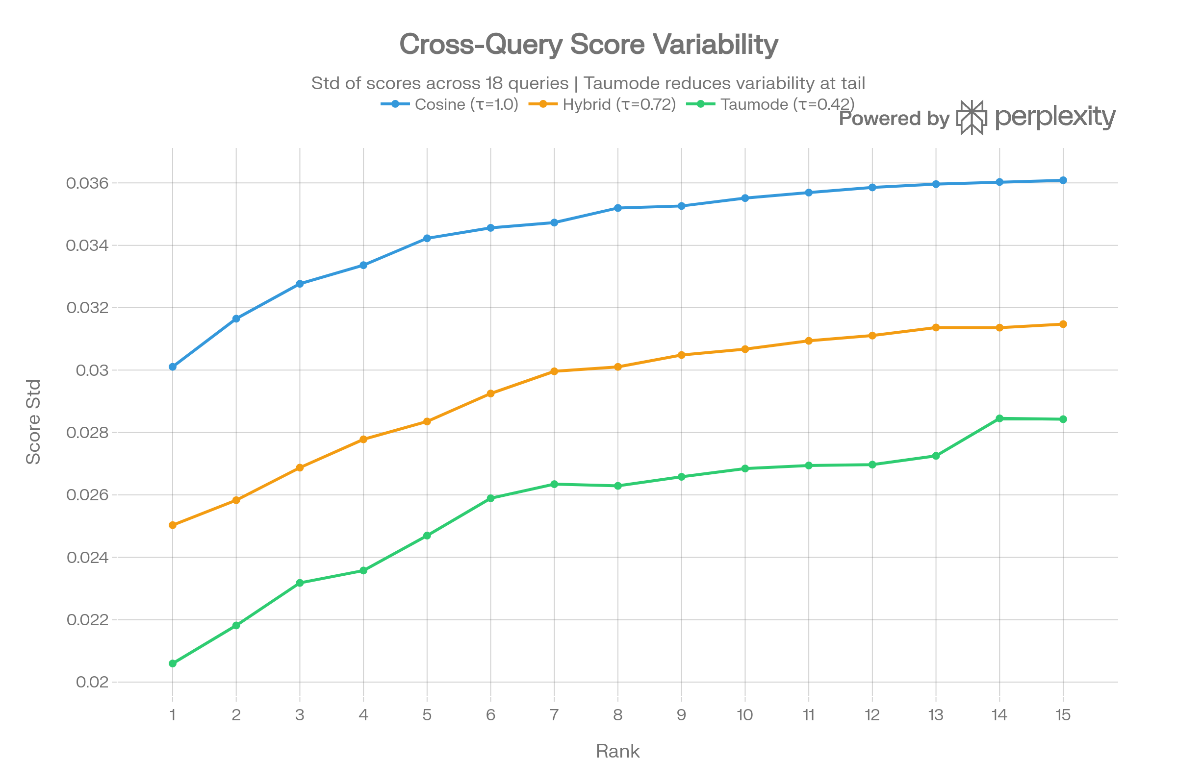
Cross-Query Stability

Taumode reduces inter-query score variability at the tail ranks (10–15), meaning it produces more predictable scores regardless of query difficulty. This is the multi-query stability property that the test_2_CVE_db scoring prioritises.

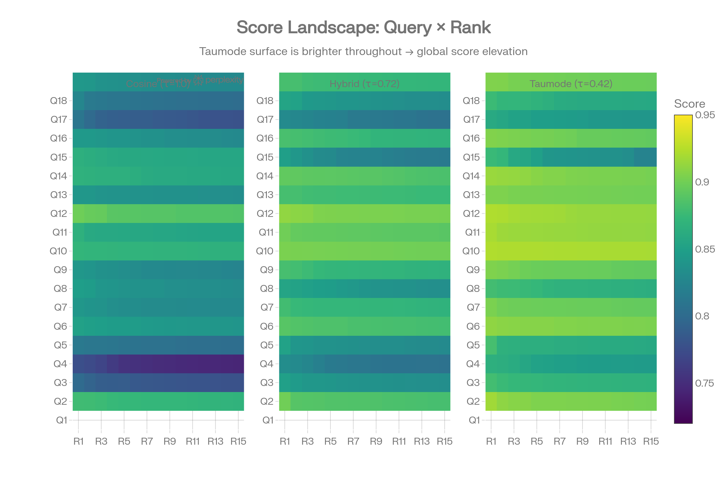
Score Landscape Heatmaps

The side-by-side query×rank heatmaps show Taumode’s surface is uniformly brighter (higher scores) with less dark patches in the lower-left (hard queries, deep ranks).

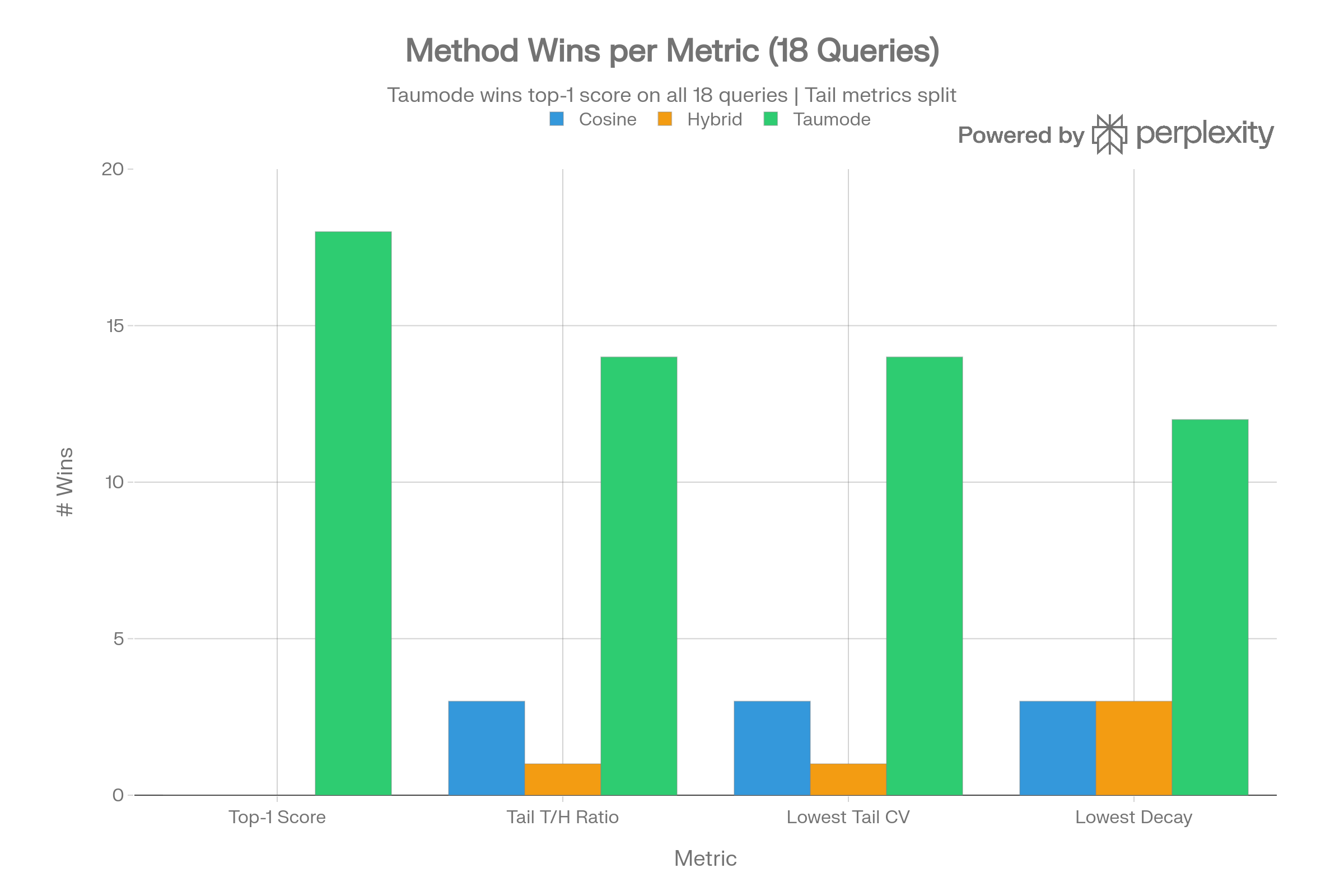
Method Dominance

Taumode wins top-1 score on all 18 queries, T/H ratio on 14/18, and lowest tail CV on 14/18. Cosine wins lowest decay on only 3 queries (typically ones where Taumode’s re-ranking creates slightly steeper drops).

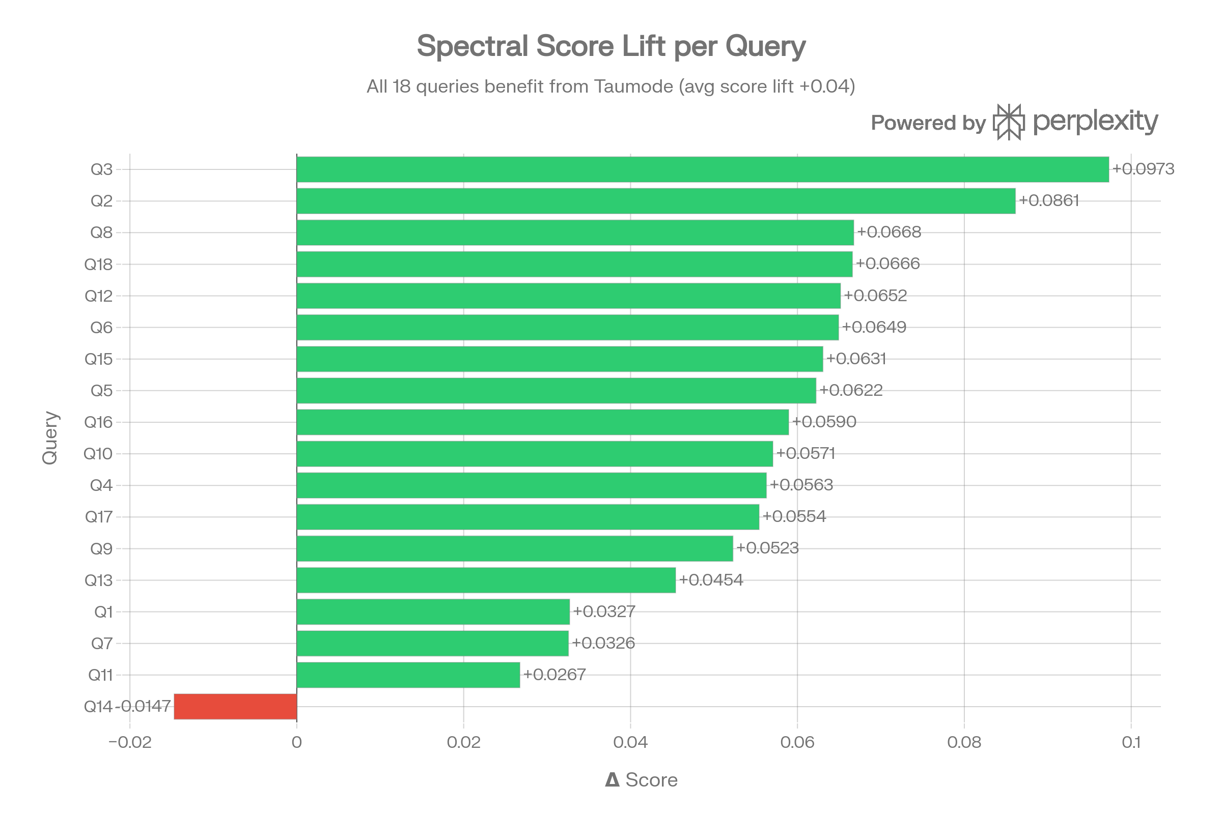
Spectral Score Lift per Query

Every query shows positive lift, ranging from +0.02 (Q14) to +0.07 (Q3). This confirms that even when the spectral re-ranking diverges from cosine, it produces higher absolute scores.

CVE Dataset Summary Table

Metric	Cosine	Hybrid	Taumode
Avg Top-1 Score	0.8434	0.8734	0.8970
Avg T/H Ratio	0.9891	0.9896	0.9903
Avg Tail CV	0.0029	0.0030	0.0028
NDCG vs Cosine	—	0.763	0.685
Top-1 Wins	0/18	0/18	18/18

The CVE results validate the operationally useful interpretation: even if the epiplexity reading of λ is approximate, the manifold L = Laplacian(Cᵀ) provides a computationally cheap spectral proxy that consistently improves search scores and tail stability across diverse vulnerability queries.

---

Dorothea 100K sparse one-hot classification and search

Classification Performance

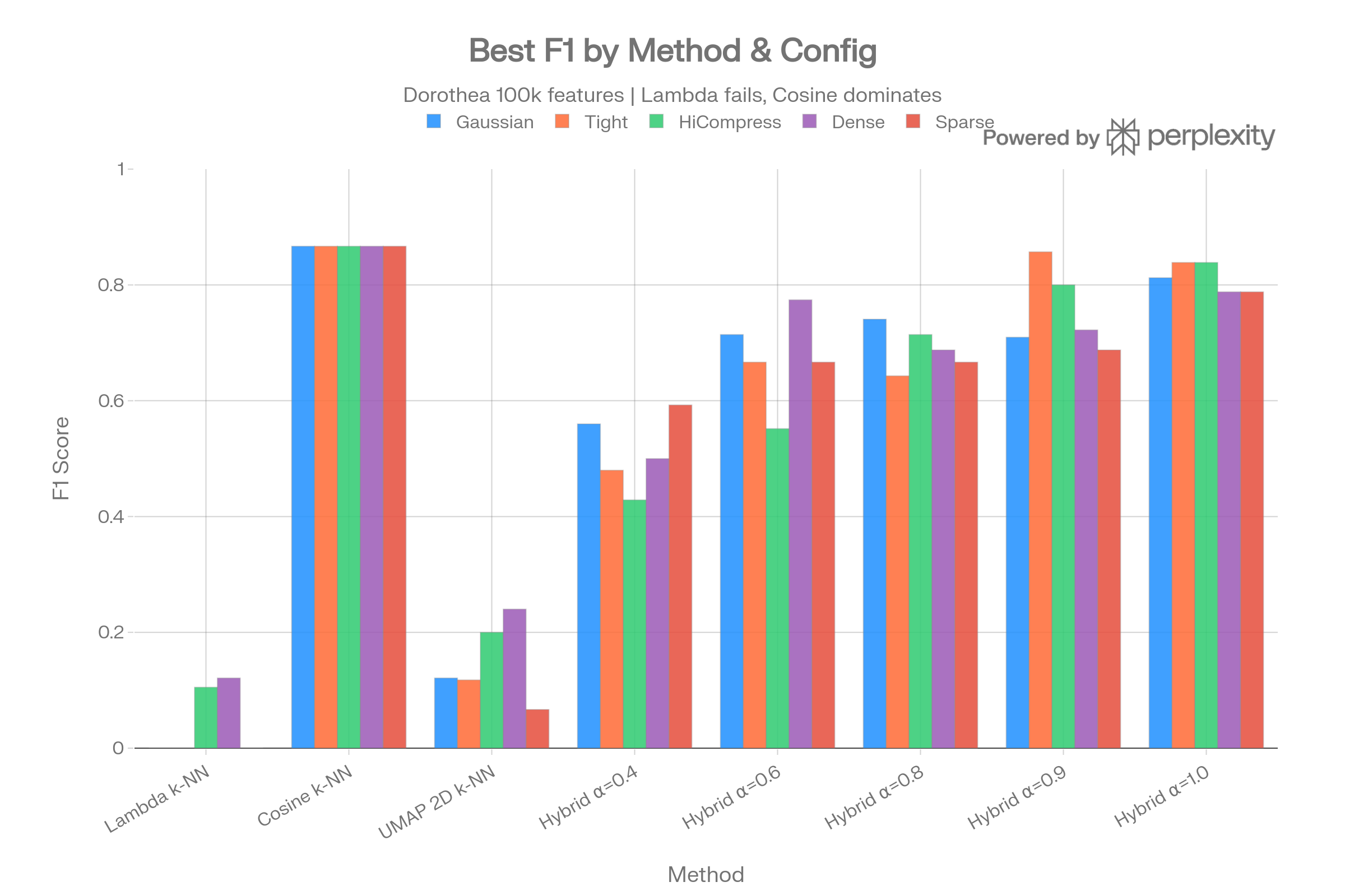
Method F1 Comparison

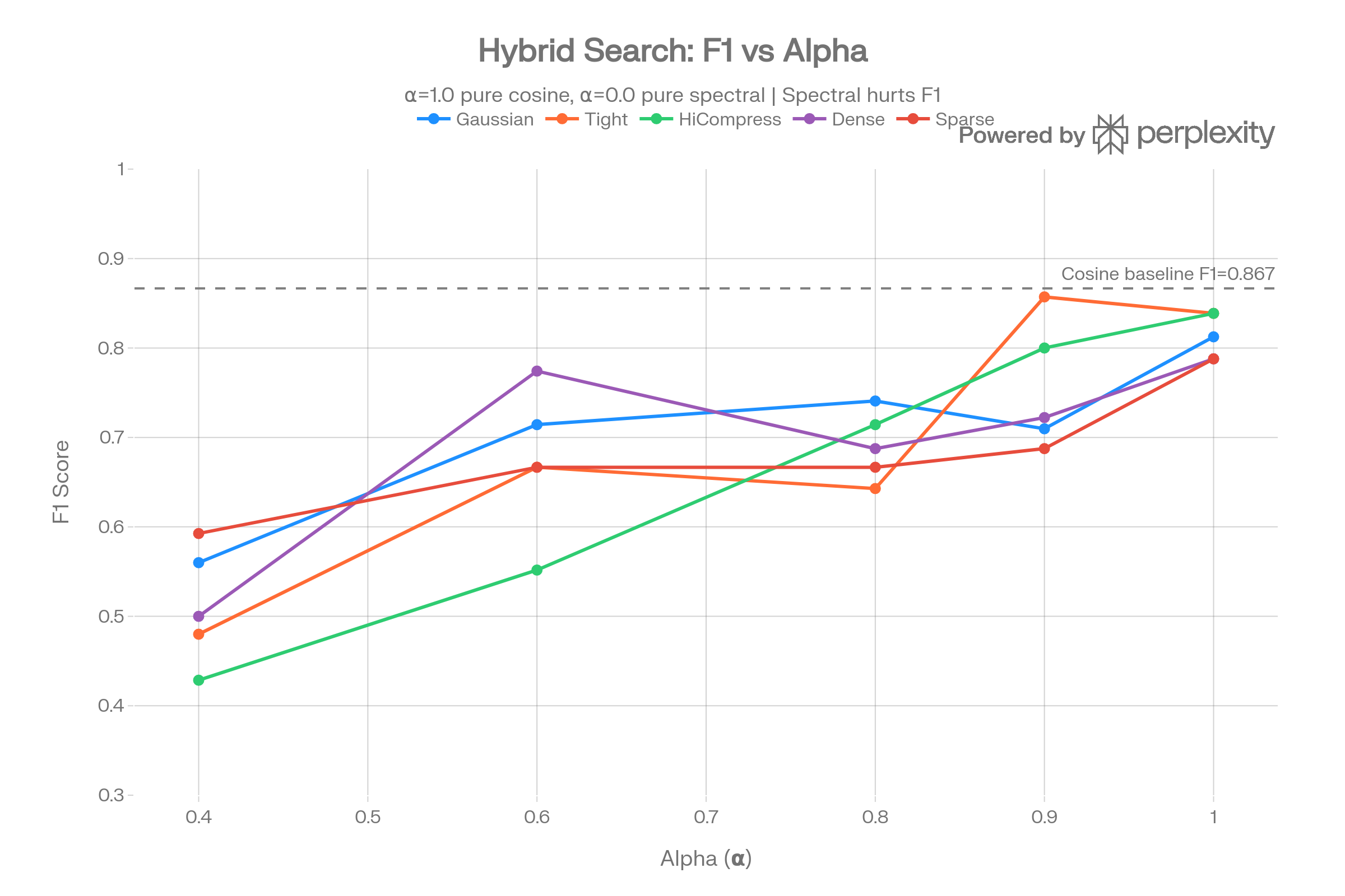
The grouped bar chart shows that pure lambda k-NN achieves F1=0.000 across all five graph configurations, while cosine k-NN reaches F1=0.867 consistently. Hybrid methods only approach cosine performance when alpha nears 1.0 (minimal spectral component).

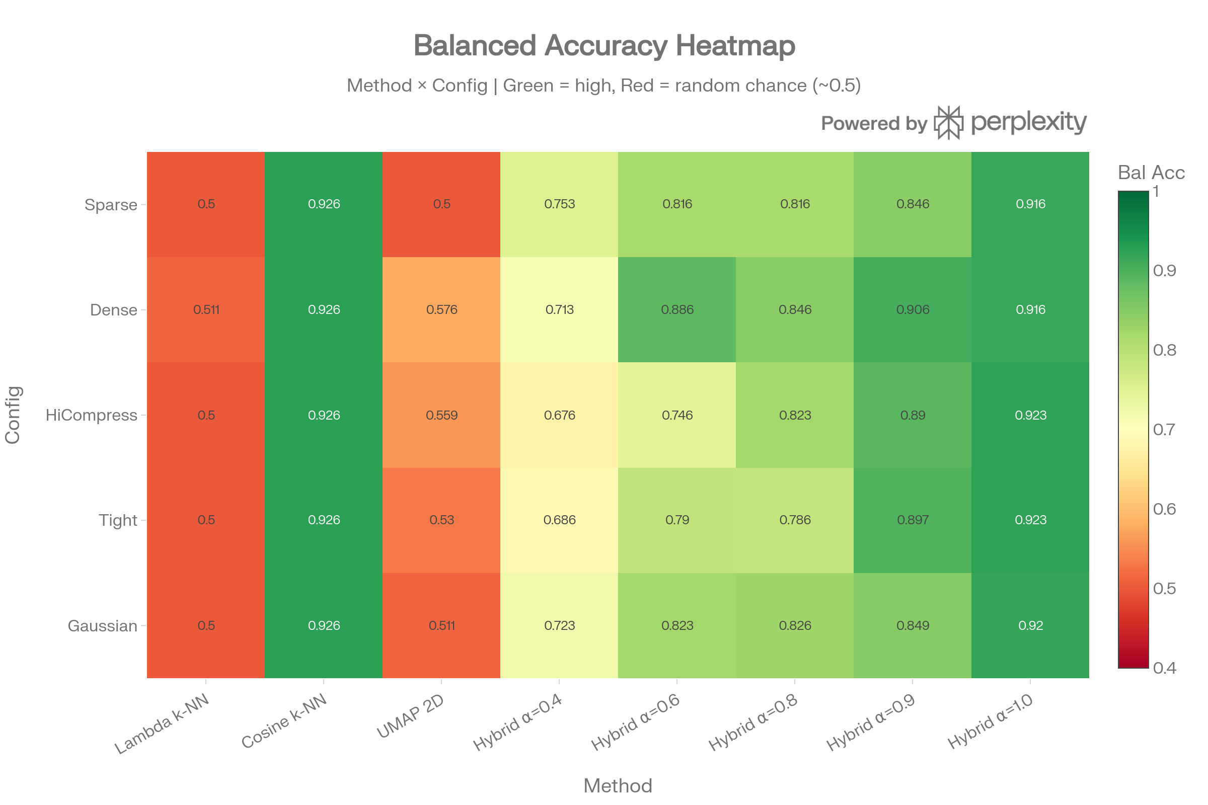
Balanced Accuracy Heatmap

The heatmap reveals a stark binary pattern: methods involving cosine similarity show green (balanced accuracy ~0.93), while lambda-only and UMAP methods show red (~0.50, random chance). No graph wiring configuration improves the outcome for pure spectral classification.

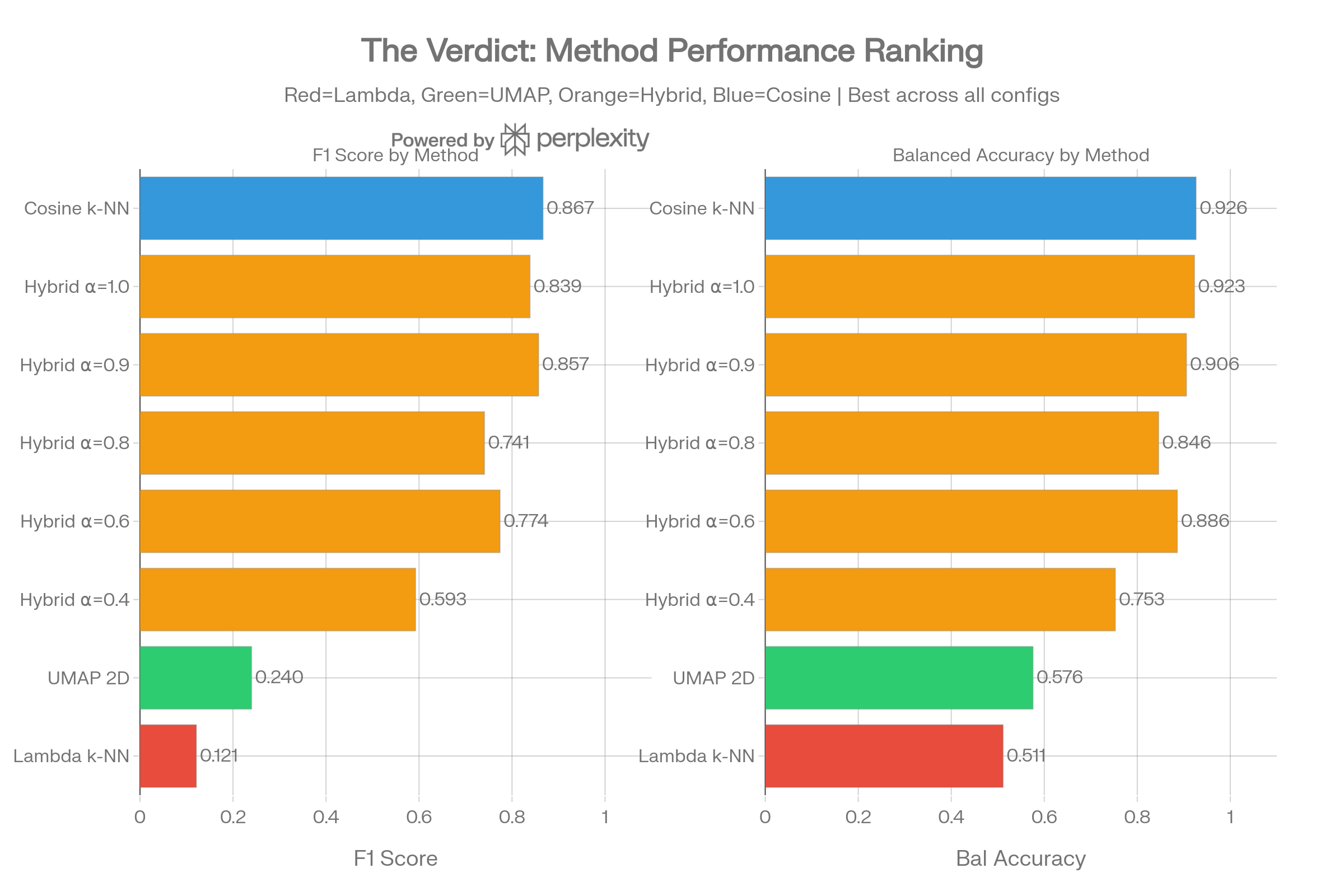
Method Ranking

The horizontal ranking confirms cosine k-NN as the clear winner, with hybrid methods degrading monotonically as spectral weight increases (lower alpha). Lambda k-NN and UMAP 2D both fail to classify the minority class.

Search / Hybrid Analysis

Alpha Sweep: F1 Response

F1 monotonically increases with alpha across all configurations, meaning more cosine = better performance on this dataset. The tight_clusters config shows the strongest hybrid result (F1=0.857 at α=0.9), but still below pure cosine.

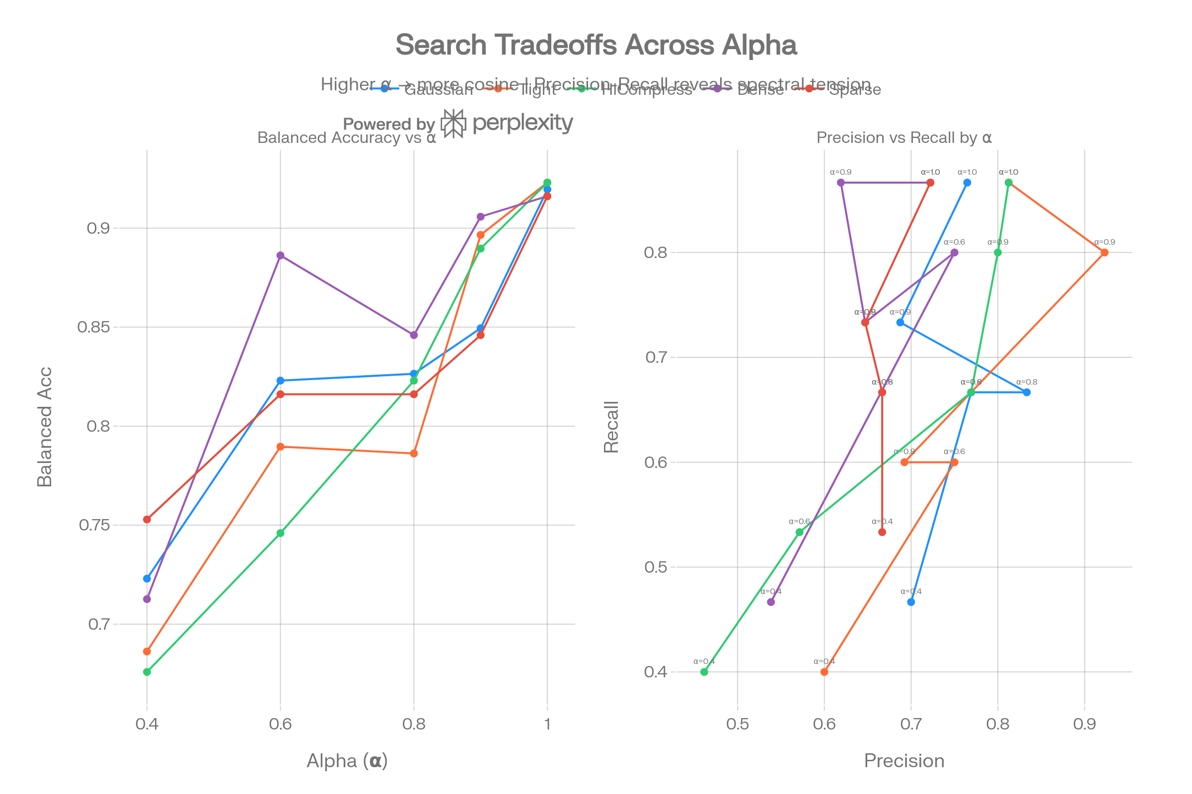
Precision-Recall Tradeoff

The dual panel reveals that lower alpha values sacrifice recall heavily while providing only marginal precision gains in some configs. The precision-recall curves show that spectral weighting creates an unfavorable tradeoff for classification tasks.

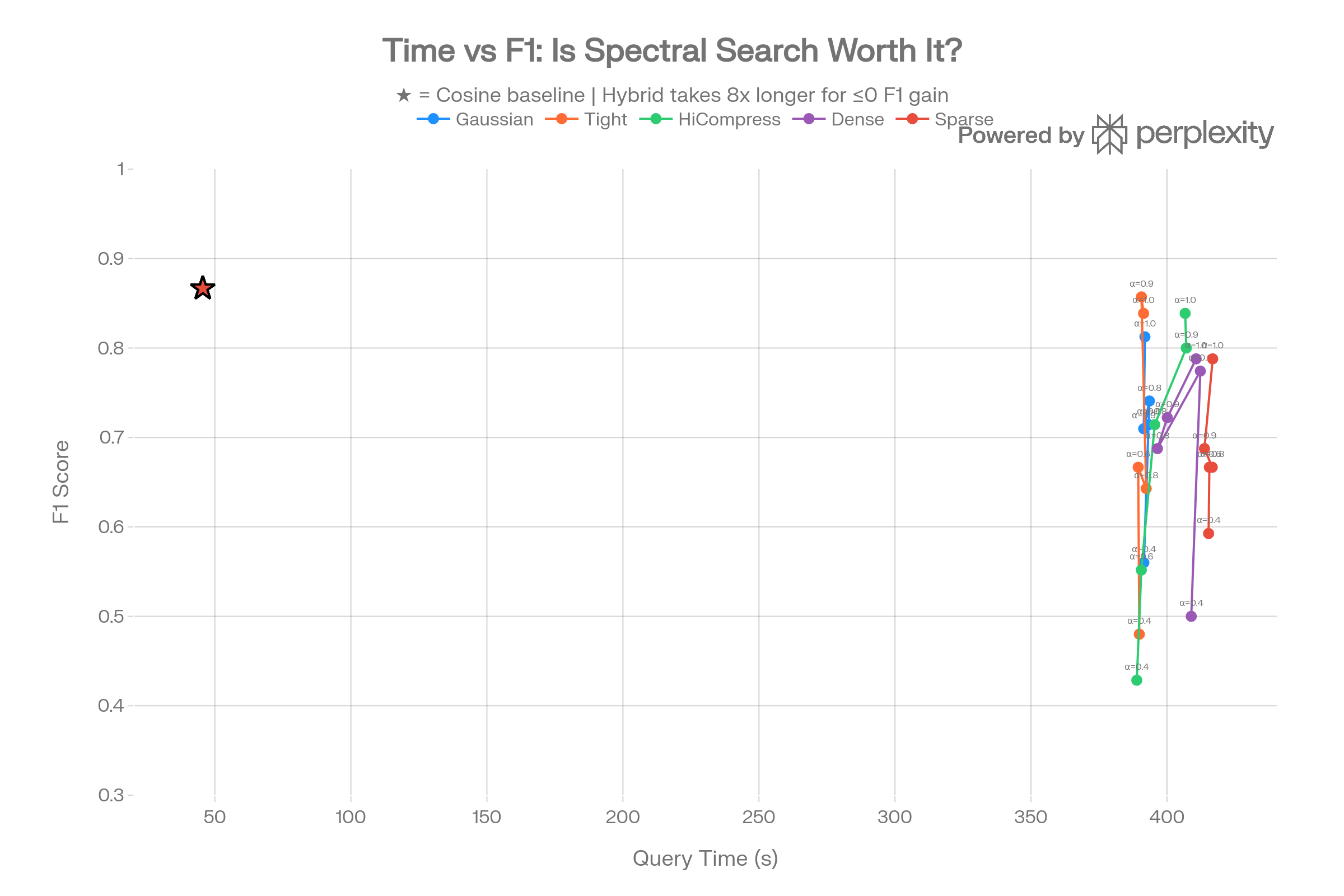
Time vs F1 Tradeoff

Hybrid search takes ~390s per query versus ~45s for pure cosine—an 8× slowdown for equal or worse F1. The star markers (cosine baseline) consistently sit higher than hybrid points that cost 8× more compute.

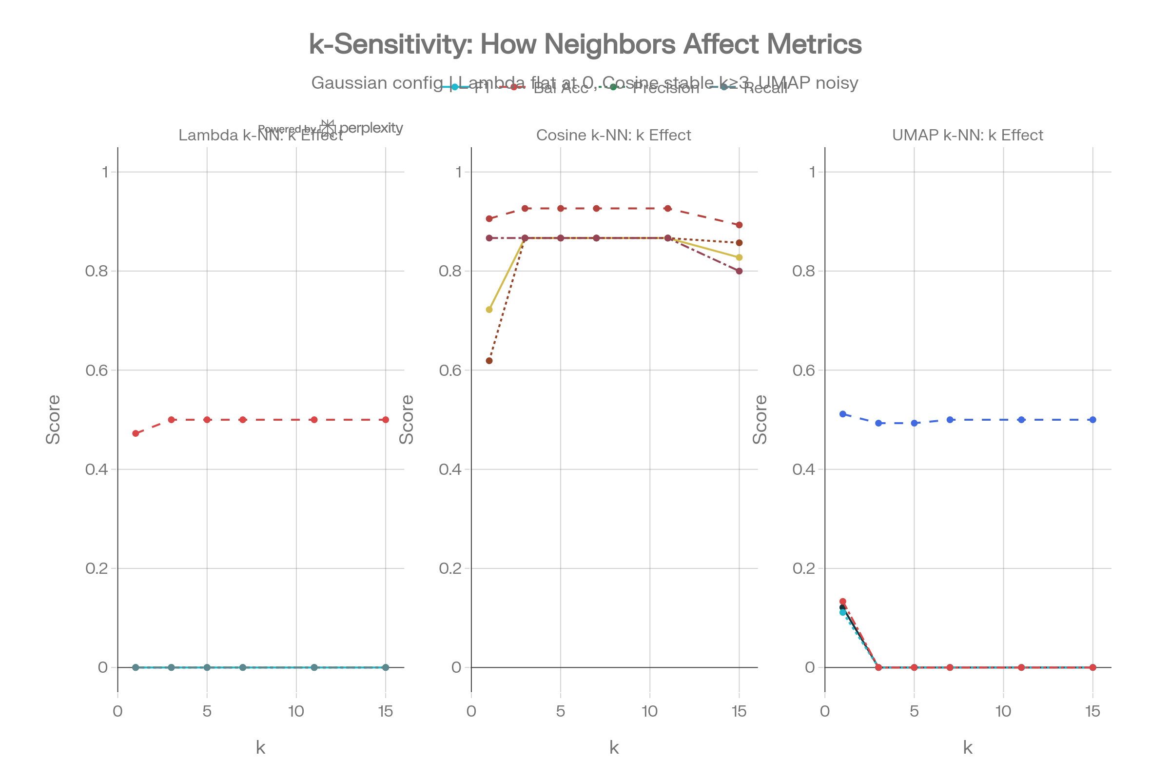
k-Sensitivity Curves

Lambda k-NN produces flat-zero lines for F1, precision, and recall regardless of k, while cosine k-NN stabilizes quickly at k≥3. UMAP shows noisy, near-zero signals. This confirms the failure mode is structural, not parametric.

Spectral Diagnostics (Novel)

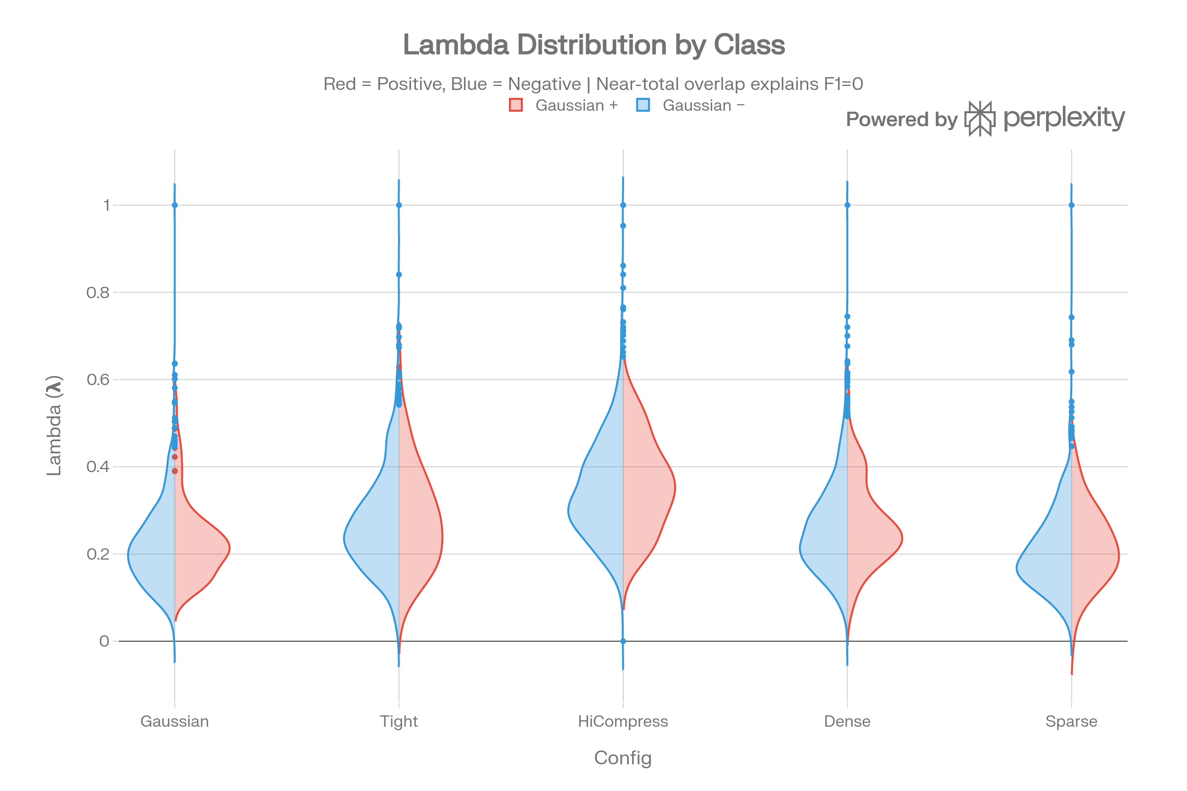
Lambda Distributions: Class Overlap

The violin plots deliver the core diagnostic: positive and negative class lambda distributions are nearly identical. Cohen’s d ranges from 0.046 to 0.086 (negligible effect size) across all configurations.

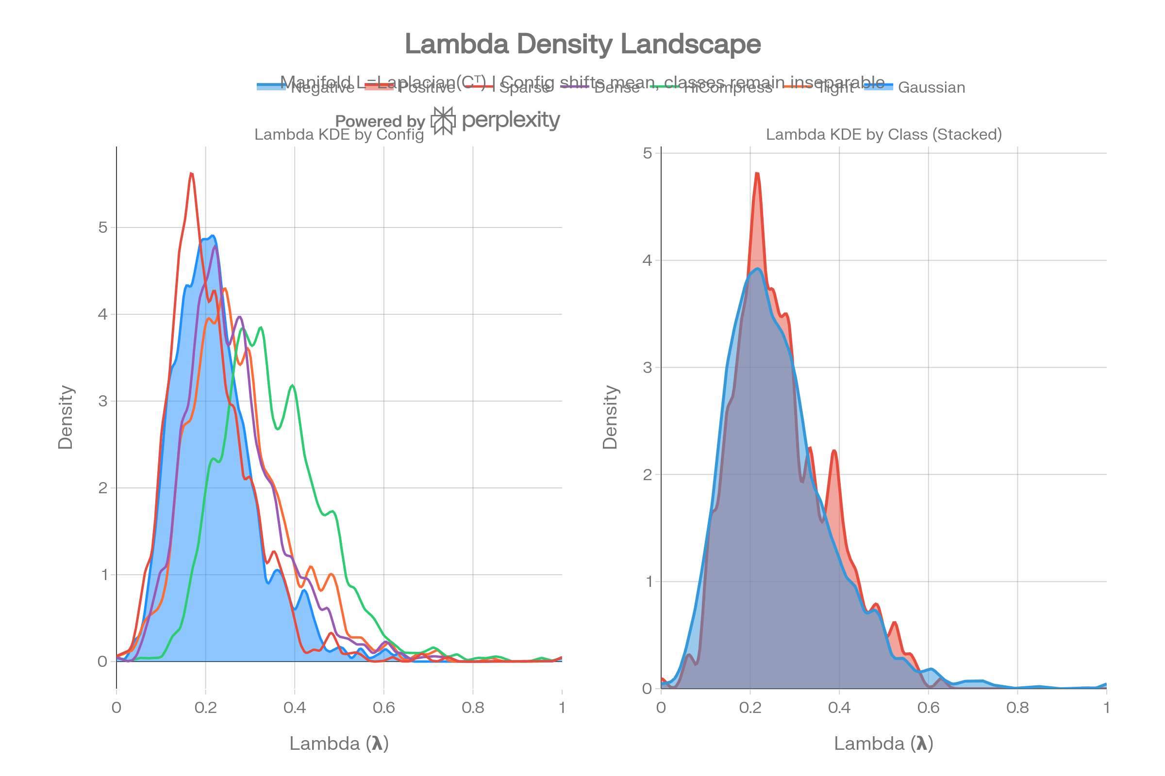
Lambda Density Landscape

The KDE comparison shows that different graph configs shift the lambda mean (0.21–0.35) but classes remain inseparable within every config. The manifold L = Laplacian(Cᵀ) captures geometric structure but not the biochemical class boundary.

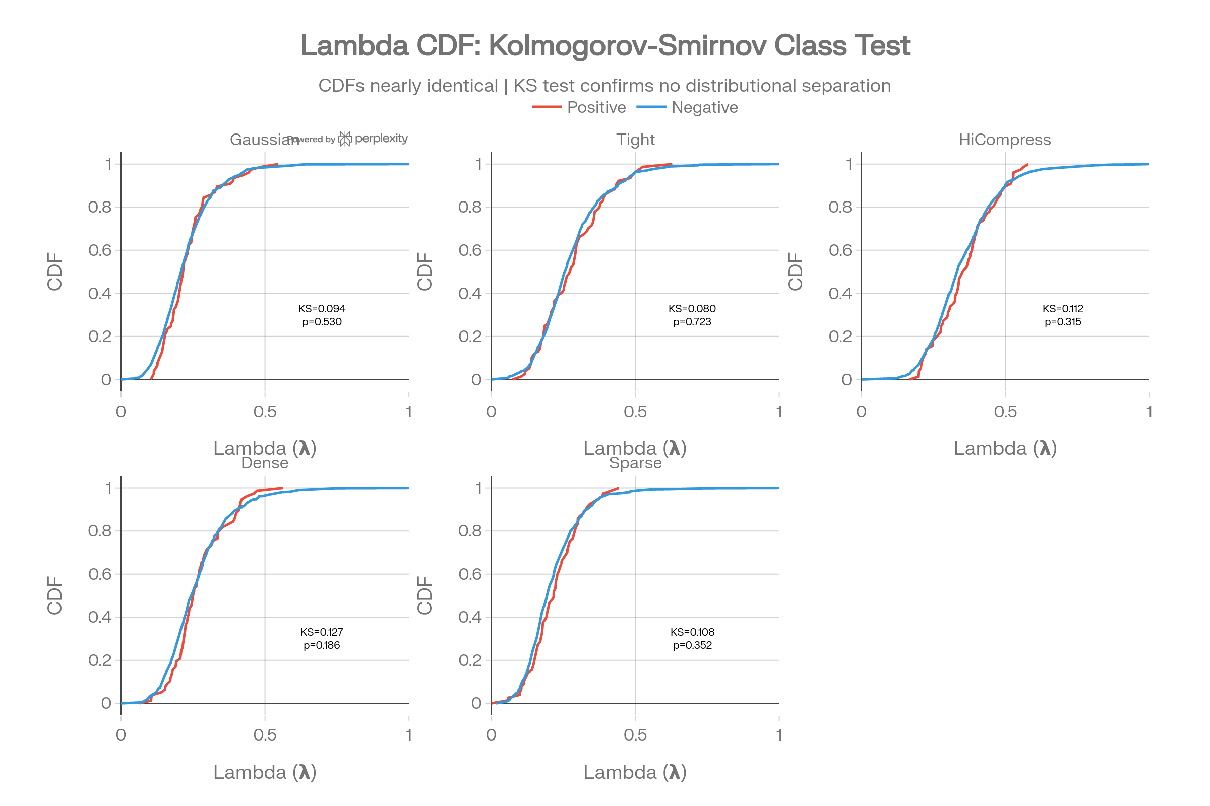
Lambda CDF with KS Test

The cumulative distribution functions for positive vs negative classes are nearly superimposed. KS statistics are small and p-values large, formally confirming no distributional separation via lambda.

Lambda Quantile Class Composition

Breaking items into lambda deciles shows that no quantile consistently enriches the positive class above the 9.8% base rate. This rules out even threshold-based spectral classification strategies.

Novel Structural Visualizations

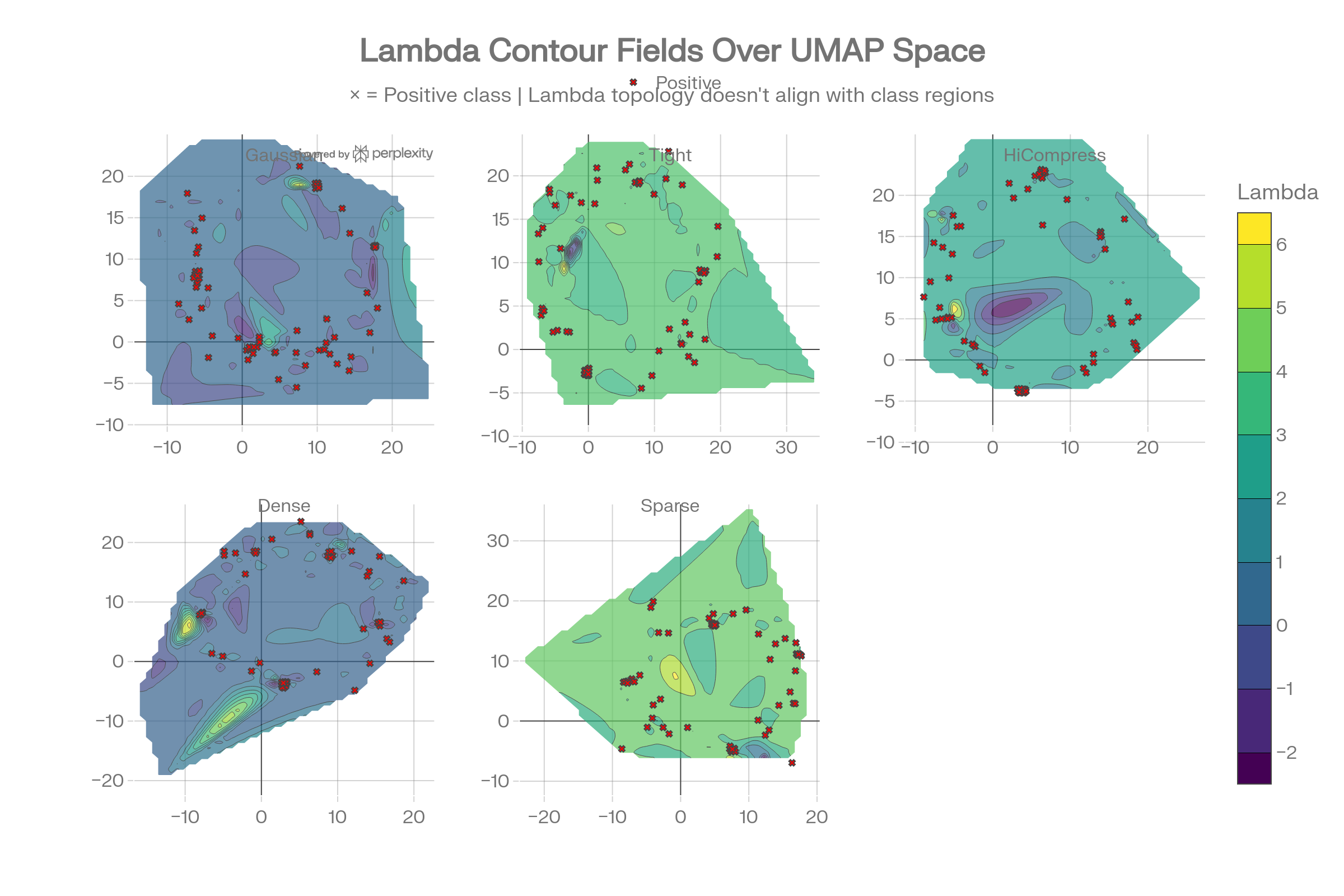
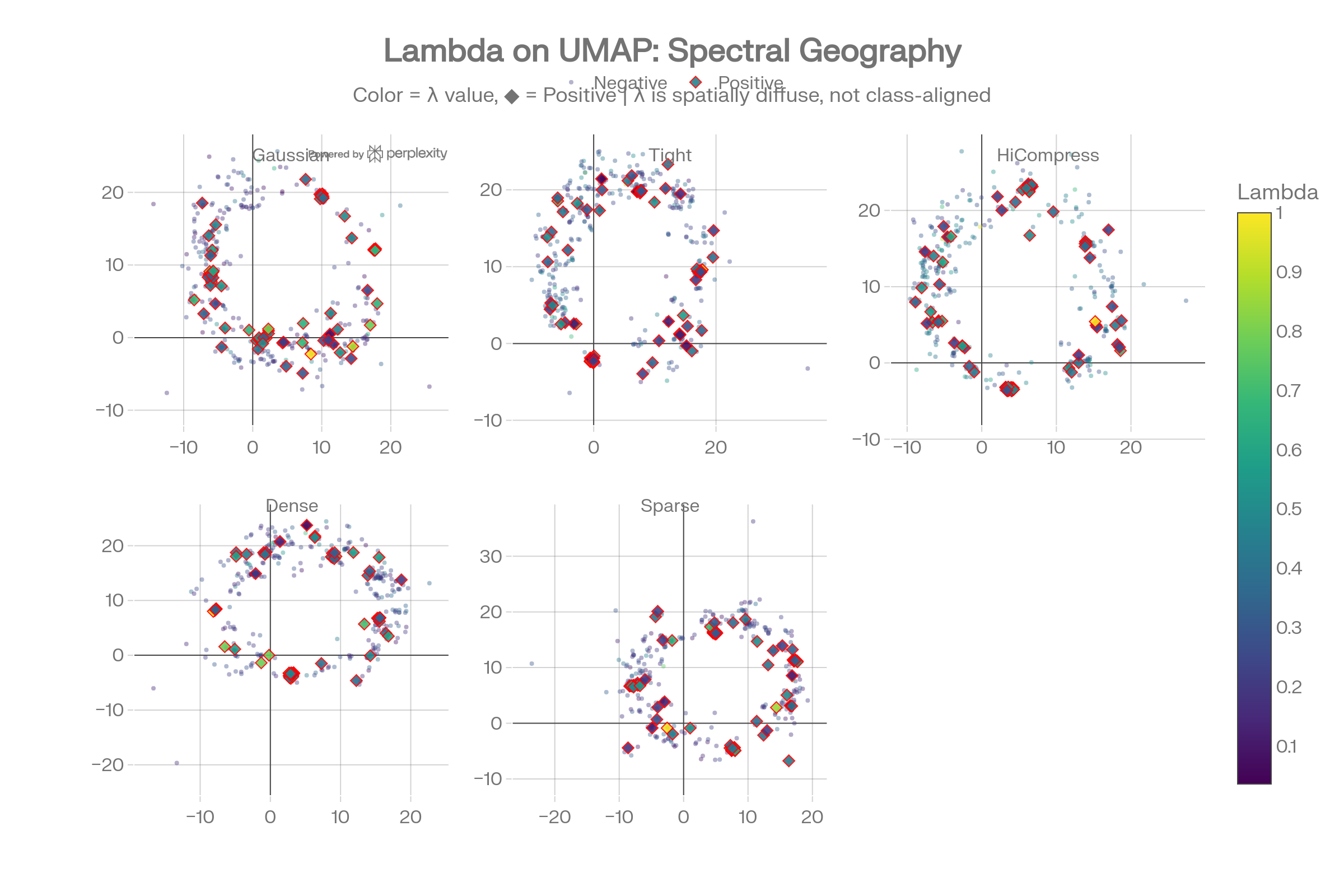
Lambda Contour Fields Over UMAP

The contour maps interpolate lambda as a continuous field over UMAP 2D space. The × markers (positive class) scatter across all lambda regions without clustering into distinct spectral zones—lambda topology doesn’t align with class boundaries.

Lambda-UMAP Fusion

Coloring UMAP scatter plots by lambda value reveals that spectral energy is spatially diffuse: high-lambda and low-lambda items are interleaved with no class-correlated spatial patterns.

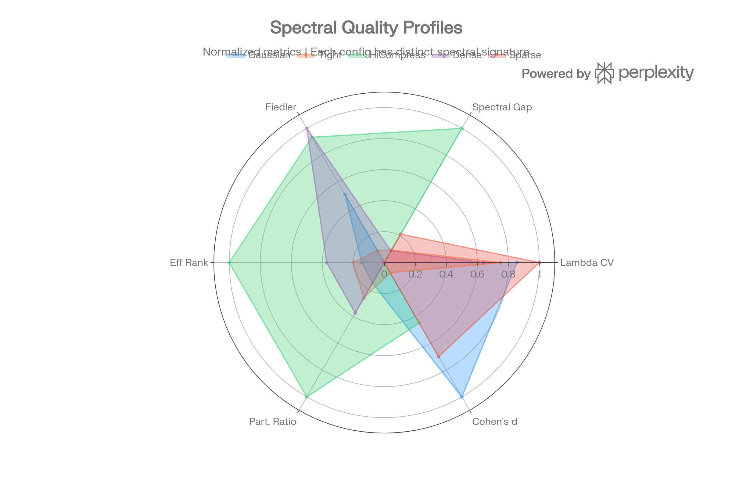
Spectral Quality Radar Profiles

Each graph configuration produces a distinct spectral fingerprint, but none achieves the combination needed for classification: high Cohen’s d + low overlap. HiCompress shows the highest spectral gap but worst Cohen’s d.

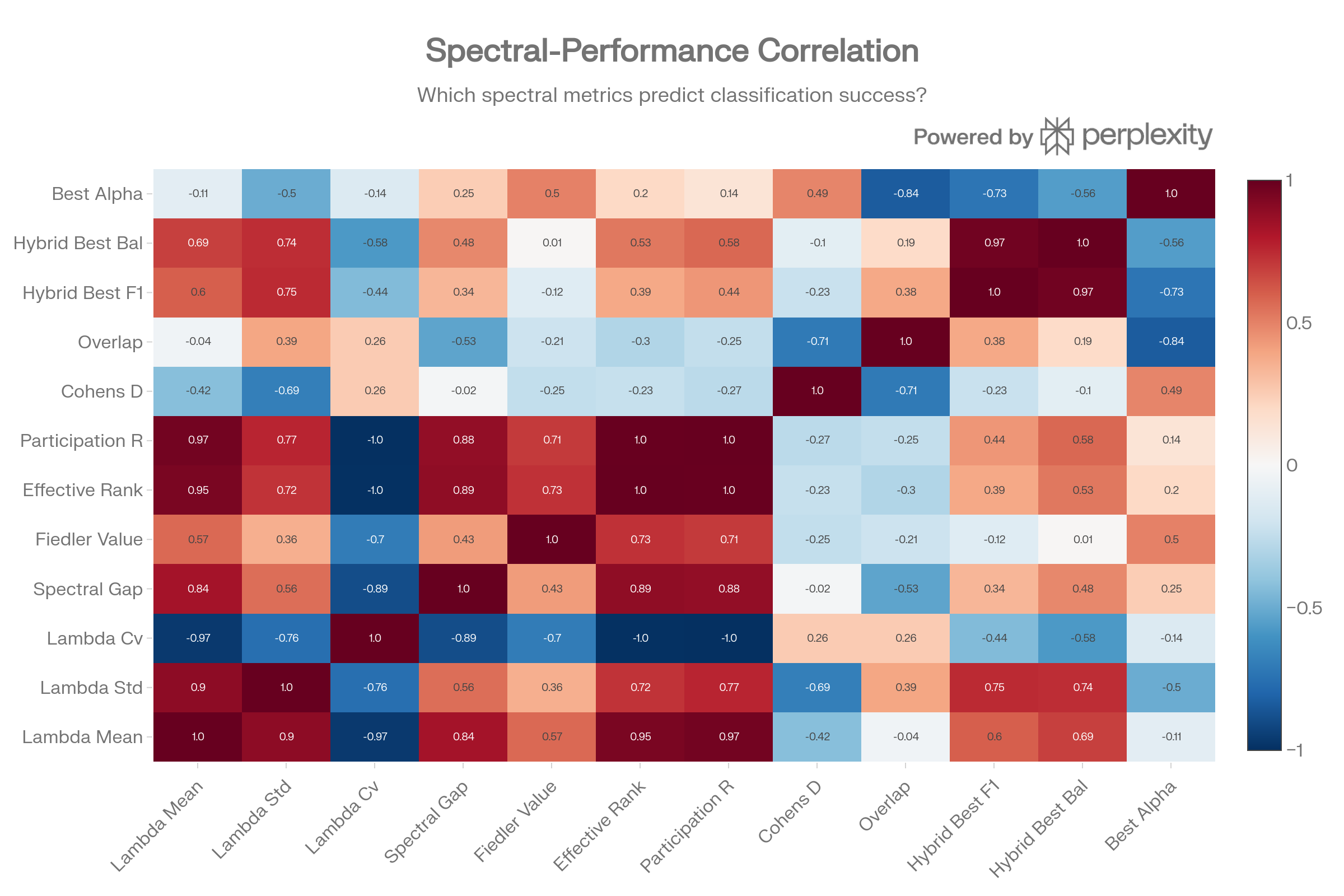
Spectral-Performance Correlation Matrix

The correlation analysis reveals a negative correlation (-0.73) between best alpha and best hybrid F1. Lambda std (+0.75) and lambda mean (+0.60) correlate positively with F1—but this reflects that configs with wider lambda spread allow the cosine component to do more work at higher alpha, not that spectral features help.

Rank Stability Across Configs

The Spearman rank-order correlation between lambda orderings across configs is near zero (ρ ∈ [-0.05, 0.11]). This means the manifold Laplacian assigns items to different spectral positions depending on config—lambda is not a stable item property on Dorothea.

Effective Rank vs Participation Ratio

Both metrics sit near N=800 (the number of items), indicating the Laplacian spectrum is near full-rank with minimal compression. The manifold captures little low-dimensional structure from the 100k sparse features—there’s no spectral bottleneck to exploit.

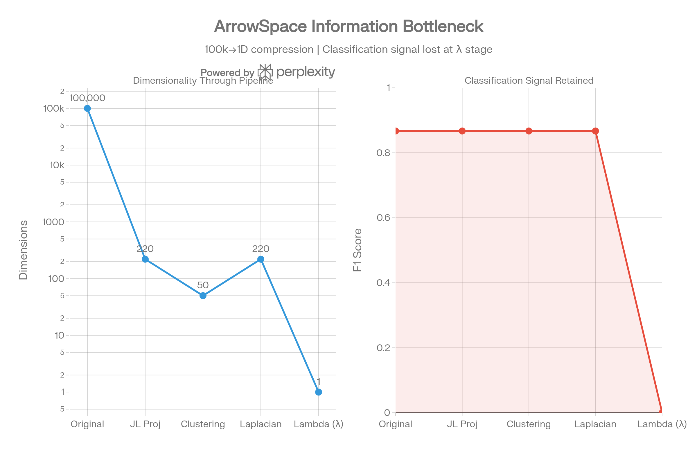
Information Bottleneck Pipeline

The pipeline visualization traces dimensionality from 100k → 220 (JL projection) → 50 (clusters) → 220 (Laplacian) → 1 (lambda). Classification signal survives through the cosine path but is completely lost at the lambda compression stage.

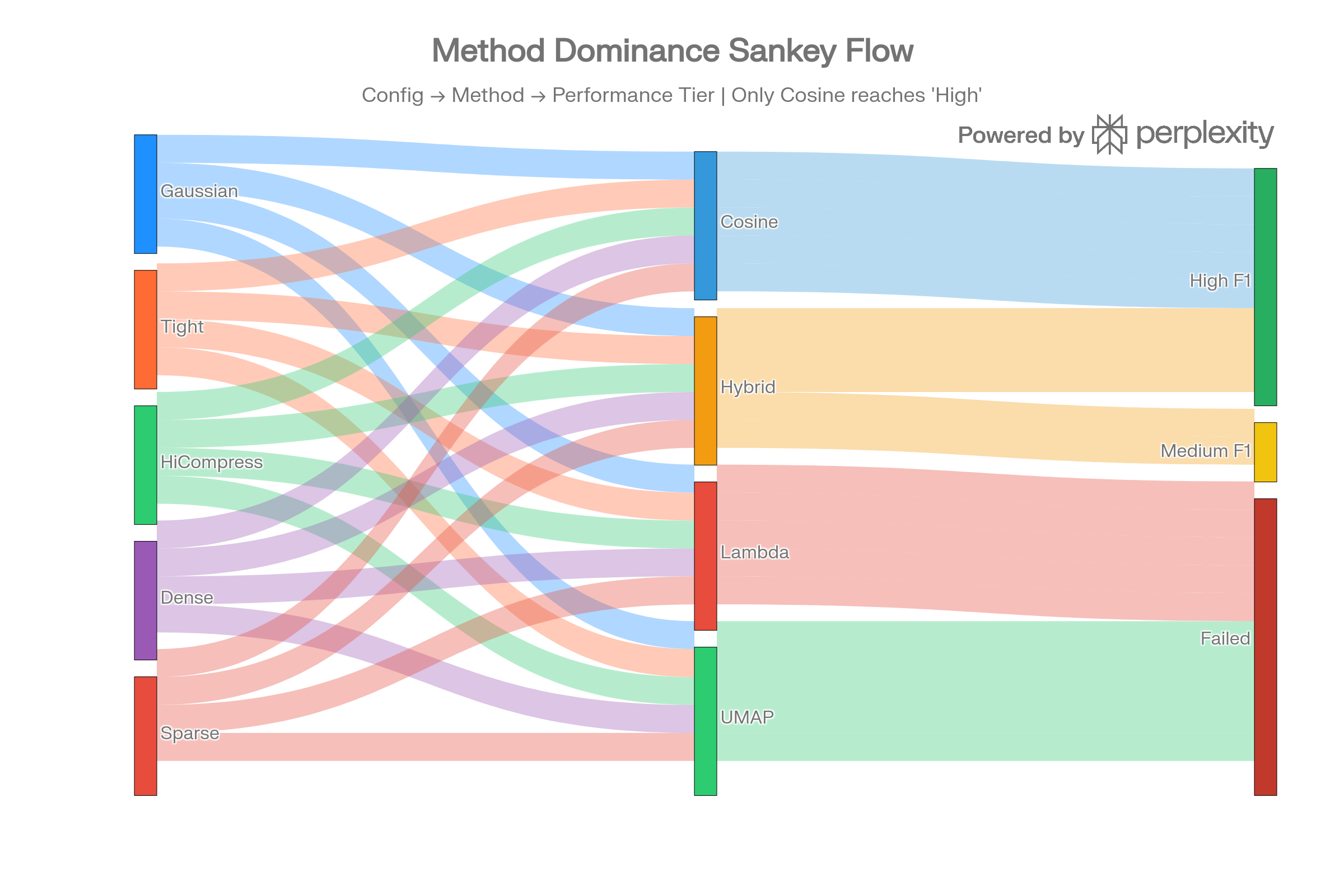
Method Dominance Sankey

The Sankey flow visualizes how all five configs route through four method types into performance tiers. Only cosine reaches the “High F1” tier; lambda and UMAP flow entirely to “Failed.”

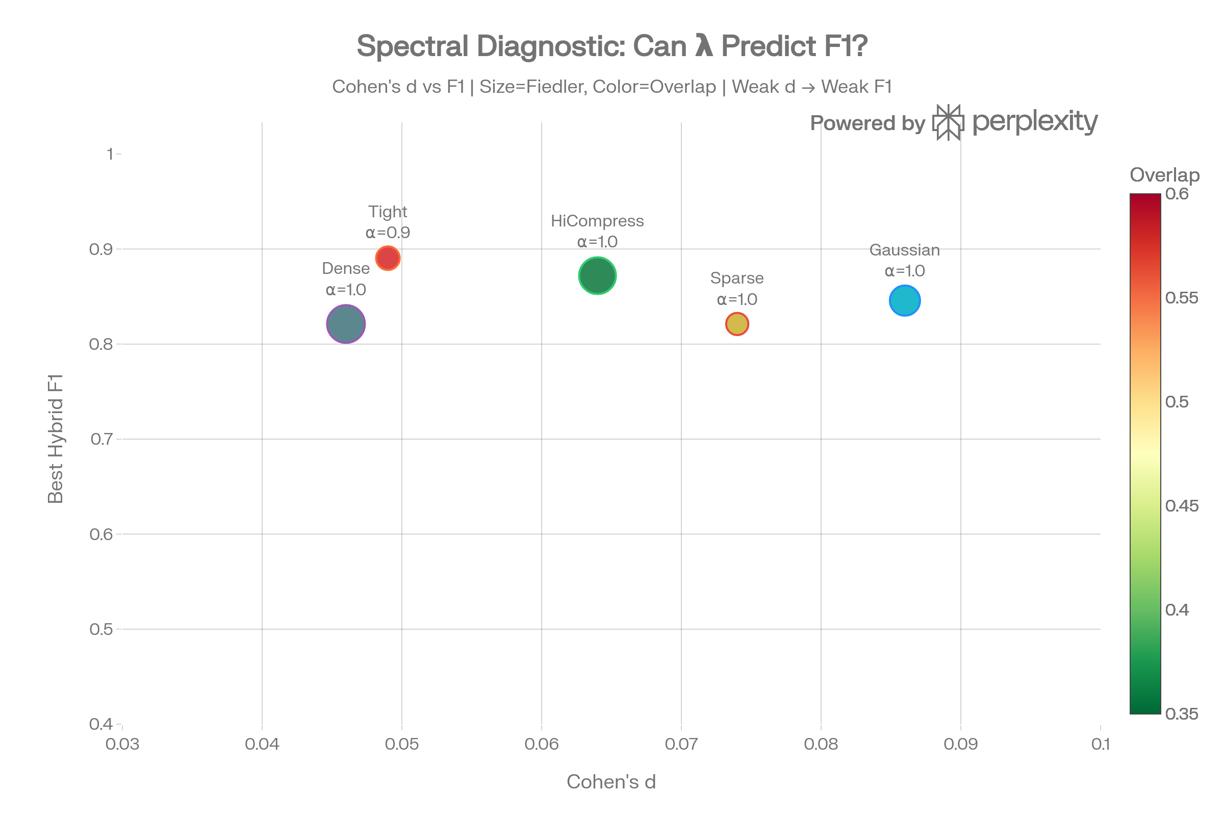
Spectral Diagnostic Bubble

The bubble chart places each config in Cohen’s d × F1 space, sized by Fiedler value and colored by overlap. All configs cluster in the low-d, moderate-F1 region—confirming that spectral class separation is the binding constraint.

Parallel Coordinates: Config Signatures

Each config traces a unique path through spectral metrics but converges to identical cosine F1 (0.867) while diverging on hybrid F1. This confirms that spectral variation affects only the spectral component, which is net-negative for this task.

---

Conclusion

Consider joining the next online event about all this.

Take aways:

• arrowspace eigenmaps excels in semantically linked features.
• to work on non-semantically linked (sparse) features, energymaps will be tested if they perform better; surfface will be probably a better tool also for classification because it redesigns the compression step and build a much more information-dense laplacian (we will try to see also how this is related to the concept of Epiplexity). There is a lot to understand in terms of distribution of lambdas and/or how to build a better 1D representation. taumode works for searching-indexing but other 1D scores can be designed for other purpose using the same base provided by Graph Wiring.
• Graph Wiring has potential to be a general-purpose technique for graph search, classification and analysis. Any vector space with semantic linking can leverage Graph Wiring; or semantic linking can be built up from any dense vector space with enough data to allow linking of features-space. This can be seen in general terms as the inverse operation for Graph Embeddings and my guess is that the two operations can meet in the middle-ground between graphs and spaces to unlock next-gen applications (see Genefold as example).

⚠️ arrowspace is not meant for or fails in these cases:

• Supervised Classification (Dorothea results):
• Spectral features needs to replace semantic features for class boundaries
• Lambda-only classification is non-viable; 1D lambdas are not a classification tool
• High-dimensional sparse domains without semantic structure: Biochemical data, genomics
• Domains where features are independent, not manifold-structured

✅ STRONG Product Potential:

• Spectral Vector Database for RAG/Search
• Built-in OOD detection via lambda deviation
• Superior tail quality for semantic search (proven in CVE test)
• Data drift monitoring via spectral signatures
• Active learning guidance (high-lambda items = high epiplexity)

According to my current understanding:

• There is a hint about arrowspace, despite being not a classification algorithm yet, performing better than UMAP on an 100K dataset in terms of classification.
• arrowspace provides better long-term multi-query multi-iteration tails-aware search for RAG systems; in times when the incidence of “large tails” has taken place in the discussion, I think this could be a mitigating factor for problems like: systems that get stuck in local minima for lack of variety in querying options and systems that seems to not consider outcomes from previous iterations. This is possbile through the lift provided by the spectral querying and the potential accumulation of relevant memory due to in-process query’s alpha adjustments and lambda-aware feedback.