arrowspace v0.21.0: proof of concept for energy-informed context search
Spectral indexing is testable
ArrowSpace v0.21.0 is a milestone release of a potential alpha-candiate that finalises the search–matching–ranking pipeline envisioned by the original `arrowspace` paper, bringing the energy-first algorithm and the eigenmaps path together into a complete POC for spectral vector search.
The release ships as the latest tag in the public repository and cements the design goal of mixing Laplacian energy with dispersion for ranking while keeping query‑time lightweight and bounded.
You can find arrowspace in the:
- Rust repository ↪️
cargo add arrowspace - and Python repository ↪️
pip install arrowspace
What’s new in v0.21.0
- The library now delivers an end‑to‑end pipeline from index build to energy‑aware retrieval, closing the loop between spectral construction and ranking as specified by the original paper’s λτ synthesis and bounded transform \(E/(E+\tau)\).
- The energy path (energymaps) is stabilized with adaptive parameters, optical compression, diffusion‑split subcentroids, energy Laplacians, and automatic λτ computation for ranking, removing cosine dependence from construction and search when desired.
Two build paths
| Path | Purpose | Core steps | Search method |
|---|---|---|---|
| build (eigenmaps) | Spectral index from Laplacians over items via eigenmaps clustering to obtain λτ per row for spectral‑aware similarity. | Cluster items, form Laplacian, compute Rayleigh energy and τ‑bounded mix to produce λτ. | search_lambda_aware and related spectral queries using λ proximity and optional cosine tie‑breaks . |
| build_energy (energymaps) | Pure energy‑first pipeline with optical compression (DeepSeek-OCR style) and diffusion that constructs an energy Laplacian and computes λτ for ranking without depending on cosine. | Clustering and projection, optical compression, diffusion and subcentroid splitting, energy Laplacian, τ‑mode synthesis on subcentroids, item‑to‑subcentroid mapping. | search_energy ranks by adaptive combination of λ proximity and bounded Dirichlet/L2 terms with automatic weights. |
Why diffusion plus splitting implies hierarchical clustering
Diffusion maps and related spectral methods naturally induce divisive hierarchical clustering because eigenvector signs and magnitudes identify blocks that can be recursively split, yielding a top‑down hierarchy on the data manifold.
Recent work (see References) explicitly couples diffusion processes with hierarchical cluster structures, showing diffusion‑conditioned or localised diffusion folders that refine clusters across levels, which aligns with ArrowSpace’s “diffuse and split” subcentroid generation used for search units.
The energymaps pipeline at a glance
Here a brief enumeration of the steps involved in the arrowspace algorithm:
- Centroids are produced by the builder’s clustering stage, with adaptive token budgeting and dataset‑aware heuristics to determine an optimal centroid count for the following steps.
- Optical compression projects centroids to 2D, bins them on a grid, trims high‑norm outliers, and pools low‑activation members—an approach inspired by DeepSeek‑OCR’s vision‑token compression that preserves structure while shrinking the candidate set.
- Diffusion smooths the centroid manifold over a bootstrap Laplacian, then high‑dispersion nodes split along local gradients to form subcentroids, creating a hierarchical, resolution‑adaptive search substrate.
- JL projection compresses subcentroid features to a target dimension derived from the builder’s reduction epsilon, ensuring projected energy scoring remains consistent across the pipeline.
- The energy Laplacian is built in reduced feature space using weighted combinations of Rayleigh, dispersion, and Dirichlet‑like terms, followed by τ‑mode λ computation on subcentroids and item‑to‑subcentroid mapping for efficient query‑time λ retrieval.
Builder controls you can use
The main building options that can be specified via the convenient ArrowSpaceBuilder are:
with_lambda_graph(eps, k, p, sigma/topk): configure the Laplacian parameters that power eigenmaps and λτ synthesis; used throughout examples and docs.with_dims_reduction(enabled, rpeps): turn on JL‑style reduction with an epsilon that the energy pipeline reuses for subcentroids to ensure projection‑aware energy scoring.with_inline_sampling(option): configure inline sampling behavior used by build flows that stage clustering or projection work.
There are more for additional fine-tuning options to characterise your dataset.
A dedicated blodpost should be focused on the eps (epsilon) as it is a critical variable that can characterise the dataset, it is the radius at which neighbours nodeas are searched for. Energy search prefers unnormalised datasets so the radius can characterise the connectivity of the dataset graph. There is work ongoing to have these parameters autocomputed at building time to provide usable starting defaults that can later be tweaked. In general the process can produce accurate statistics about the nature of the dataset that can be used for comparisons like for example: what happens to this dataset if I remove this slice of items? How this two shapshots taken at different times differ? How these differences affects potential data drifting in my model? arrowspace can be seen as an integrated tool for searching, matching and ranking with powerfull dataset analysis capabilities for your data operations.
Building the index
⚙️ build: constructs the index and computes λτ over the item graph, enabling λ‑aware search and range queries immediately with familiar methods shown across the project.
ArrowSpaceBuilder::new().build(rows)
🚀 build_energy: runs clustering, compression, diffusion‑split, JL projection, energy Laplacian construction, τ‑mode on subcentroids, and item mapping in one call.
ArrowSpaceBuilder::new()
    .with_dims_reduction(true, Some(rpeps))       // dims_reduction is mandatory
    .build_energy(rows, EnergyParams::default())  // η (eta) is defined here
How to query with search_energy
Once the index is built, the search-ranking-matching can be run with search_energy(query, gl_energy, k):
queryis a query vector in the shape of the original datasetgl_energyis the graph Laplacian as computed at build timekis the number of results required from the search.
This operation computes the query’s λ once via subcentroid mapping and ranks results by an adaptive energy distance that blends λ proximity with a bounded feature‑space term, returning the best k matches, relying on cosine only at the very last stage when tie-breaking of ranking is needed. The method auto‑tunes weights from stored λ statistics and warns on degenerate ranges, keeping ranking robust while preserving the “only lambdas at query‑time” footprint emphasized in prior posts.
Storage and footprint
After construction, only per‑item λ values (1-D), the lightweight norms (1-D) and the reduced sparse graph Laplacian (sparse matrix on FxF) need to be kept for energy search; the heavy graph structures used during synthesis can be discarded or reused offline, which keeps the runtime index compact and easy to persist alongside vectors.
This design makes serialization straightforward because ranking at query time works on a scalar λ plus a small projected feature computation, rather than requiring graph traversal or reconstruction.
The next step is to provide querying also from the parquet file so to avoid keeping the original dataset in memory, it will be interesting to see the perfomance gap. This can open the perspective of running this kind of search at datalake scale.
EnergyParams: η (eta)
To use build_energy a new set of parameters is necessary (fear not, defaults generation of also these parameters is planned). η (eta) controls how aggressively the diffusion operator updates centroid features during each iteration of the smoothing process. The update formula is:
where \(L\) is the bootstrap Laplacian and \(x\) is the centroid feature vector. This is a discretised heat equation that smooths the centroid manifold over the graph structure defined by \(L\).
How it works in the pipeline
During the diffusion and split stage, arrowspace applies eta for a specified number of steps to smooth centroid positions following the edges of the bootstrap Laplacian graph. After diffusion completes, high‑dispersion nodes split along local gradients to form subcentroids, creating the hierarchical search substrate.
The main parameters are:
- eta: step size per iteration (default 0.1)
- steps: number of diffusion iterations (default 4)
Values tested in the benchmark sweep
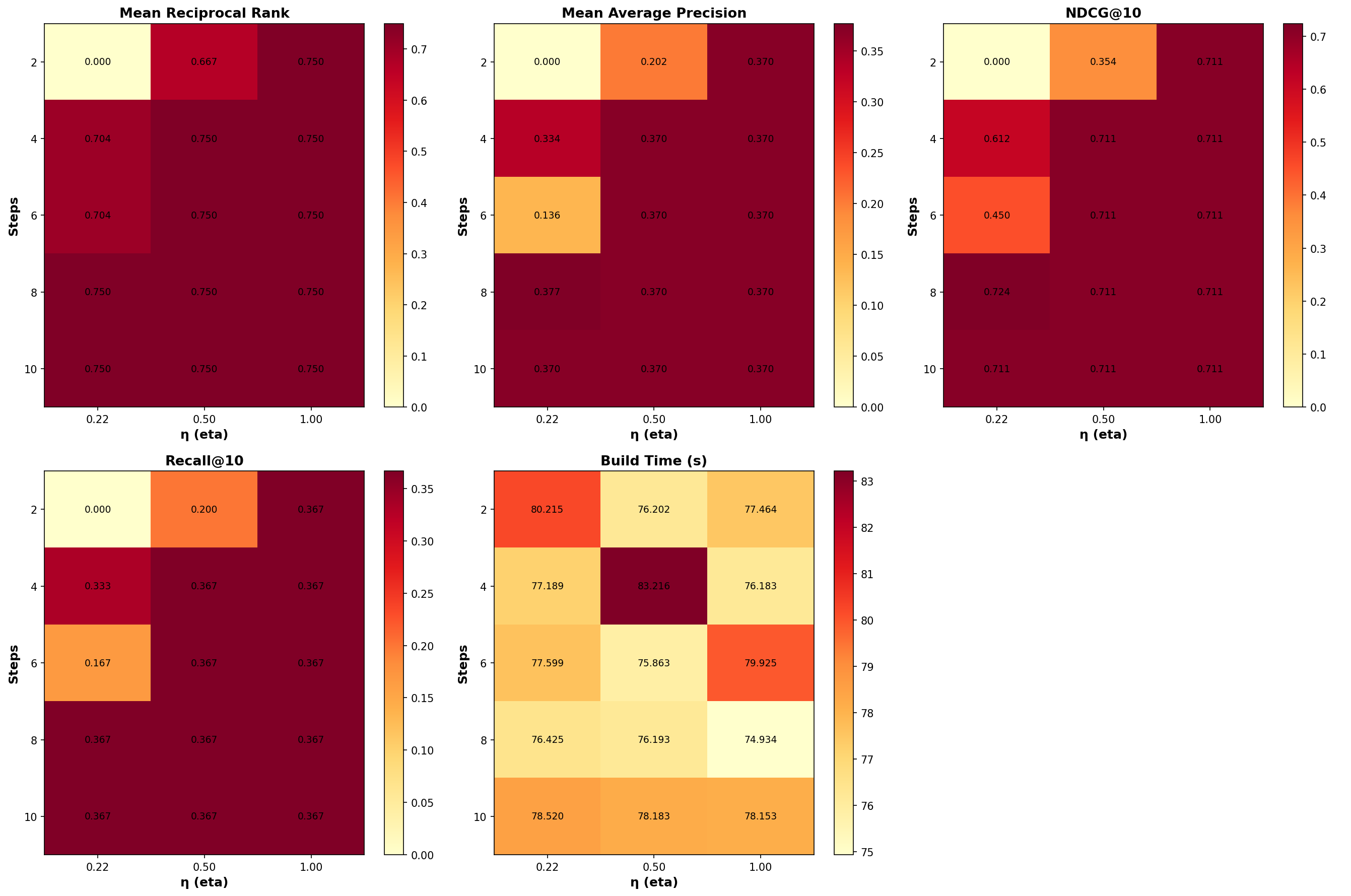
The CVE benchmark below swept eta across three values: \(0.22\), \(0.5\), and \(1.0\), combined with steps in \({2, 4, 6, 8, 10}\).
Key observations from the sweep:
- eta=0.22, steps=8 delivered the highest Avg MRR (0.75) and best NDCG@10 (0.7239), indicating moderate diffusion with sufficient iterations captures the manifold structure effectively.
- eta=0.5, steps=4 also achieved Avg MRR 0.75 and is flagged as the best trade‑off between accuracy and build speed in the blog post, with build time of 83.22s.
- Higher eta values (0.5, 1.0) with more steps converged to similar metrics (MRR 0.75, NDCG 0.7106), suggesting the manifold reaches a stable state after moderate smoothing.
- Lower eta with fewer steps (η=0.22, steps=2) produced degenerate results (MRR 0.0), indicating insufficient diffusion to establish meaningful graph connectivity.
Tuning guidance
- Smaller eta (0.1–0.3) requires more steps to achieve the same smoothing effect but provides finer control over convergence.
- Larger eta (0.5–1.0) smooths faster but risks overshooting or homogenizing the manifold if steps are too high.
- The default (η=0.1, steps=4) balances speed and stability for most datasets, but the benchmark suggests η=0.22–0.5 with 4–8 steps works well for large embeddings like the CVE corpus.
Why it matters
Eta directly influences how much local graph structure gets incorporated into the subcentroids that serve as search units. Too little diffusion leaves noisy, disconnected clusters. Too much diffusion over‑smooths and loses discriminative topology. The sweep confirms that moderate η with sufficient steps produces stable, high‑quality energy rankings while keeping build times under 85 seconds (for 300Kx384 dataset on a 12 core machine).
Benchmarks at a glance
I have run a sweep on the CVE corpus (300K documents with 384 dimensions recording common vulnerabilities discovered in software systems since 1999). The figure below shows stable build times around 75–83 seconds across \(η\) (energy parameter) in \({0.22, 0.5, 1.0}\) and optical compression steps in \({2, 4, 6, 8, 10}\), indicating diffusion overhead is negligible relative to construction.
- The best aggregate observed in this sweep is \(η=0.5\) with steps=4 as best trade-off between accuracy and building speed.
- Heatmaps summarizing MRR, MAP, NDCG@10, Recall@10, and build time visualize how low‑η with moderate steps tends to deliver strong ranking quality in this dataset while keeping build times uniform.
Test Queries
Three domain-specific queries probe different vulnerability classes:
- “authenticated arbitrary file read path traversal”
- “remote code execution in ERP web component”
- “SQL injection in login endpoint”
Metrics
Standard IR metrics are computed@20:
- MRR (Mean Reciprocal Rank): Quality of top-1 result
- MAP@20 (Mean Average Precision): Ranking quality across all relevant items in top-20
- NDCG@10 (Normalized Discounted Cumulative Gain): Graded relevance with position discount
- Recall@10/20: Fraction of relevant items retrieved
Results
Style note and prior context
- The energymaps work extends the previously documented optical compression and energy search article, where text‑as‑image compression inspired the 2D binning and pooling primitive that now ships as the default compression stage in the energy pipeline.
- The JOSS paper formalizes λτ and its bounded transform \(E/(E+\tau)\), which this release operationalizes end‑to‑end for search–matching–ranking, completing the original vision with a robust builder API and stabilized energymaps.
Why this matters
- v0.21.0 provides a practical spectral index that finds matches beyond geometric proximity by encoding manifold structure directly in the index, not just in a reranker, as demonstrated in the paper and examples.
- The combination of diffusion‑driven hierarchical refinement, τ‑bounded energies, and compact λ‑only querying unlocks discovery of relevant alternatives while preserving top‑rank fidelity, matching the goals set out in prior posts and tests
Please consider sponsoring my research and improve your company’s understanding of LLMs and vector databases.