ArrowSpace for Latent Spaces — part 3
A companion notebook is available.
In part 2, I used ArrowSpace to study transformer representations as dual geometric and semantic objects: token neighborhoods in item space, and operator-induced structure in feature space. The result was not just a list of “important layers” but a map of layer-role subspaces where semantic structure sharpens, especially along the dual/readout side of the model. That analysis exposed something important and I am going to extend it here leveraging part of the theory defined in Intelligence From Learnable Novelty pre-print paper.
A low-energy basin is not automatically a useful basin. Some basins are smooth because they contain meaningful, compressible structure. Others are smooth because they are trivial: locally regular, easy to predict, and mechanically uninteresting. If mechanistic analysis is meant to tell us where the model is doing useful internal work, then smoothness alone is not enough.
This suggests a sharper question for Part 3:
Can epiplexity separate trivial basins from useful basins inside a given subspace or transition zone?
The question comes from a recent paper on learnable novelty, which proposes epiplexity as a quantity that rewards structure that is surprising enough to matter but regular enough to be learned. That distinction matters here. ArrowSpace already gives me a way to locate local basins and spectral transition zones. Epiplexity may provide a second filter: not “where is the geometry smooth?” but “where is the geometry smooth in a way that still contains learnable structure?”
What epiplexity actually measures
The paper decomposes the total description length of a dataset \(Y\) given \(X\) into two parts:
\[L^\phi(Y \mid X) = \underbrace{|M_\phi^*|}_{\text{epiplexity } S^\phi} + \underbrace{(-\log_2 p(Y \mid X, M_\phi^*))}_{\text{unlearnable residual } H_T}\]The first term, \(S^\phi\), is the learnable novelty: the program length of the best model a bounded observer \(\phi\) can fit. The second, \(H_T\), is the residual the model can never reduce. A noisy television contributes only \(H_T\); a dark room contributes neither. Maximising \(S^\phi\) alone avoids both failure modes.
The paper gives a closed-form reservoir estimator that makes this cheap and differentiable. A fixed random nonlinear map (the reservoir) produces features \(\tilde H\); all learnable capacity resides in a linear ridge readout whose optimum is closed-form:
\[W_\lambda = (\tilde H^\top \tilde H + \lambda I_m)^{-1} \tilde H^\top \tilde Y\]The epiplexity is the spectral description length of \(W_\lambda\):
\[S^\phi(Y \mid X) = \frac{1}{2} \sum_i \log_2\!\bigl(1 + \eta\, s_i(W_\lambda)^2\bigr)\]where \(s_i\) are the singular values of \(W_\lambda\). Each independent learnable direction in the
readout contributes bits; redundant or spurious directions contribute only logarithmically.
A stronger ridge \(\lambda\) suppresses spurious structure (chance correlations that a bounded learner
cannot actually exploit). The epiplexity Python library (pip install epiplexity) implements
this framework: a TTimeProbabilisticModel interface and an EpiplexityEngine that computes both
\(S_T\) (structural bits) and per-item \(H_T\) (entropy bits), with an ArrowSpaceModelAdapter
that bridges ArrowSpace’s feature-space Laplacian to a Laplacian-constrained Gaussian MRF.
ArrowSpace and Epiplexity are not globally correlated, as if they were two imperfect thermometers for the same hidden variable. That would be too blunt, and it would probably miss the actual mechanistic opportunity. The more useful question is local and operational:
- Is a basin merely low-energy?
- Or is it also a site where the model has created useful learnable structure?
- Can that distinction help identify better targets for inspection, intervention, or ablation?
A revised definition of semantic basin
Part 2 treated semantic basins primarily through local spectral structure: low Laplacian energy, coherent neighborhoods, and field-selective concentration in certain layer-role subspaces. For Part 3, I want to tighten that definition.
A semantic basin will no longer mean just a locally smooth region in one ArrowSpace view. Instead, I will treat it as the cross-section of two signals:
- ArrowSpace locality — a neighborhood is spectrally coherent in item space and/or feature space.
- Epiplexity — the same neighborhood supports learnable structure rather than mere regularity or noise.
Under this definition, a basin becomes interesting only when both conditions hold.
That immediately rules out two failure cases:
- Trivial basin: low spectral roughness, low epiplexity.
- Noisy boundary: high roughness, low learnability.
What remains is the more interesting case:
- Useful basin or transition zone: local coherence combined with non-trivial learnable structure.
This is the object I actually care about for mechanistic analysis.
Why global correlation would be the wrong target
Part 2 already showed that semantic behavior is not uniformly distributed. It is concentrated in particular subspaces: specific layers, specific matrix roles, and especially the dual/readout directions where the model’s learned structure becomes easier to decode. If that is true, then a single global correlation coefficient is likely to flatten the very pattern I want to study.
So the protocol for Part 3 is deliberately local.
I want to rank neighborhoods within a subspace, compare those rankings across probes and check whether epiplexity helps discriminate between:
- smooth but uninteresting regions,
- noisy and unstable regions,
- and structured, inspectable regions where the model seems to be doing useful semantic work.
That is a mechanistic question, not a population-average one.
Concrete protocol
The plan is as follows.
Protocol pipeline: ArrowSpace locality feeds epiplexity scoring, which filters to useful basins.
1. Re-run Part 2 at token level
Part 2 already works at the level of layer-role subspaces, and it already distinguishes:
- Probe A vs Probe B,
- primal/write vs dual/read,
- embeddings vs internal operators.
The first change is simple but important: re-run the analysis at the token level, not just as field means.
The objective is to keep local structure visible rather than averaging it away too early.
2. Build local neighborhoods per token and subspace
For each token in each projected subspace, construct a local \(k\)-nearest-neighbor neighborhood.
For each neighborhood, compute local ArrowSpace descriptors in both views:
- item-space spectral descriptors,
- feature-space spectral descriptors,
- local roughness or smoothness,
- and any local energy quantities already used in Part 2.
This replaces one global \(\lambda\) per field with a local basin profile per token-neighborhood pair.
3. Define two epiplexity tasks
I want to use epiplexity in two distinct ways.
Cross-space learnability
Define:
- \(X =\) local item-space coordinates (PCA of the \(k\)-NN neighbourhood),
- \(Y =\) local feature-space vectors (the embedding rows for those items).
The cross-space score is the reservoir epiplexity of predicting features from geometry:
\[S_{\mathrm{cross}} = S^\phi(Y_{\mathrm{features}} \mid X_{\mathrm{coords}}) = \frac{1}{2} \sum_i \log_2\!\bigl(1 + \eta\, s_i(W_\lambda)^2\bigr)\]where \(W_\lambda\) is the ridge readout from reservoir features of \(X\) to \(Y\). The question here is whether the local geometry of neighboring items predicts the local semantic-feature pattern in a learnable way. A trivial low-rank basin produces \(W_\lambda\) with few significant singular values (low \(S_{\mathrm{cross}}\)); a useful rich basin produces many (high \(S_{\mathrm{cross}}\)).
Operator learnability
Define:
- \(X =\) pre-operator representation (token direction before the weight matrix),
- \(Y =\) post-operator representation (the projected vector after \(W\)).
The operator score is the reservoir epiplexity of predicting the output from the input:
\[S_{\mathrm{op}} = S^\phi(Y_{\mathrm{post}} \mid X_{\mathrm{pre}}) = \frac{1}{2} \sum_i \log_2\!\bigl(1 + \eta\, s_i(W_\lambda^{\mathrm{op}})^2\bigr)\]The question here is whether a specific operator subspace is transforming inputs into outputs in a way that is not merely regular, but learnably structured. This second score is especially relevant for mechanistic analysis, because it attaches learnability directly to the transformation performed by the model.
4. Rank, do not regress
Within each layer-role subspace, rank neighborhoods by:
- ArrowSpace local basin score,
- \(S_{\mathrm{cross}}\),
- \(S_{\mathrm{op}}\),
- contextual lift between Probe A and Probe B,
- and read/write asymmetry where relevant.
Then compare the rankings using:
- top-\(k\) overlap,
- Spearman rank agreement,
- stability across probes,
- and concentration of high-scoring neighborhoods inside known semantically sharp subspaces.
This is better than forcing a single Pearson correlation across all points. I am not looking for a universal scalar law. I am looking for useful local agreement.
5. Prioritize FFN readout and late-layer dual subspaces
Part 2 already suggests where the most informative structure sits: late-layer readout directions, especially on the dual side.
So the first target is not “all subspaces equally.” The first target is:
- FFN readout,
- late-layer readout,
- and other subspaces where Part 2 already showed semantic sharpening.
If epiplexity adds value anywhere, it should add value there first.
Working hypotheses
This protocol gives me four immediate hypotheses.
H1. Global correlation may stay weak, but local agreement may appear inside the right subspaces
A weak global correlation would not be a failure.
The stronger prediction is narrower: inside the semantically active subspaces, local epiplexity rankings may align with ArrowSpace basin rankings even if the whole model does not show one clean cross-space trend.
H2. Probe B should increase epiplexity where Part 2 already showed semantic sharpening
If Probe B is actually surfacing more usable semantic structure, then the neighborhoods highlighted by Probe B should show increased learnable novelty, not just increased dispersion.
This matters because it distinguishes sharpening from mere scattering.
H3. The best mechanistic sites are not the smoothest ones overall
The most useful regions may be the neighborhoods with:
- strong epiplexity lift,
- tolerably low feature-space roughness,
- and stable local coherence.
That is a stricter condition than “low \(\lambda\).”
H4. Epiplexity is more useful as a filter for intervention targets than as a universal basin score
This may be the most important hypothesis.
If epiplexity helps rank which subspaces or neighborhoods are worth ablating, probing, or tracing, then it is already useful — even if it never becomes a universal semantic-basin metric.
That would still be a win for mechanistic analysis.
A three-way basin typology
If this works, it gives a more precise vocabulary than Part 2 alone.
Each local neighborhood can be placed into one of three regimes:
| Regime | ArrowSpace profile | Epiplexity profile | Interpretation |
|---|---|---|---|
| Trivial basin | Smooth / low roughness | Low | Regular but mechanically uninteresting |
| Noisy boundary | Rough / unstable | Low | Surprising but not learnable |
| Useful basin | Locally coherent | High | Structured and learnable; strong intervention target |
This is the distinction I was missing before. ArrowSpace alone is good at locating structure. Epiplexity may help decide whether that structure is actually worth mechanistic attention.
The three-way typology. The useful basin (top-left) is the cross-section of ArrowSpace locality and epiplexity: smooth enough to be coherent, rich enough to be learnable.
Demonstration: the typology on synthetic data
A companion notebook
(07_arrowspace_basins_epiplexity_typology.ipynb) demonstrates the typology on three synthetic
regimes in \(\mathbb{R}^{32}\):
- Trivial — a rank-2 smooth ellipse: smooth but only two learnable directions.
- Useful — a rank-8 smooth manifold: smooth AND rich in learnable structure.
- Noisy — i.i.d. isotropic Gaussian: rough, no learnable structure.
The notebook uses both the epiplexity library’s ArrowSpaceModelAdapter (LGMRF bridge, confirming
property P7: smooth signals have lower \(H_T\) than rough signals on the feature-space Laplacian) and
a ReservoirEpiplexity model (the closed-form estimator from eq 9, implemented as a
TTimeProbabilisticModel subclass and run through the same EpiplexityEngine).
The reservoir estimator cleanly separates the three regimes:
| Regime | Roughness | \(S^\phi\) | \(H_T\) | Typology |
|---|---|---|---|---|
| Trivial | 0.012 (low) | 4.5 (low) | 3.7 (low) | smooth but uninteresting |
| Useful | 0.062 (low) | 8.5 (high) | 45.9 (mod) | smooth + learnable ← target |
| Noisy | 0.481 (high) | 6.2 (mod) | 59.2 (high) | rough, not learnable |
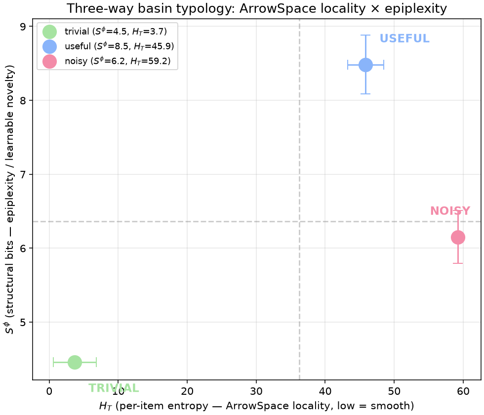
The \((H_T, S^\phi)\) plane. The useful basin (blue) sits high on the epiplexity axis while remaining low on roughness — the cross-section that matters for mechanistic analysis.
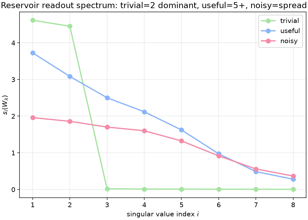
Singular value spectrum of \(W_\lambda\) per regime. The trivial basin has two dominant directions (its rank-2 ellipse); the useful basin spreads across five; the noisy regime’s apparent structure is spurious — suppressed by the ridge but still visible as a flat, low spectrum.
The key result (hypothesis H3 below): the best mechanistic sites are not the smoothest ones overall. The trivial basin is smoothest, but the useful basin trades a little roughness for much higher learnable novelty. ArrowSpace locality alone cannot make that distinction; epiplexity can.
What success would look like
A successful result would not be “epiplexity correlates with everything.”
A successful result would look more like this:
- late readout subspaces contain neighborhoods with strong local rank agreement,
- Probe B increases epiplexity where semantic sharpening already appears,
- and the top-ranked neighborhoods are better ablation candidates than neighborhoods selected by smoothness alone.
That would justify redefining semantic basin as a joint object: local spectral coherence plus local learnable novelty.
What failure would still teach
A null result would still be informative.
If epiplexity fails to separate useful basins from trivial ones, then that is evidence that ArrowSpace’s notion of basin structure and epiplexity’s notion of learnability are not aligned in these subspaces. That would not kill either framework. It would simply mean they are tracking different properties.
That is still valuable, because mechanistic analysis depends on getting the distinctions right.
Why this matters for ArrowSpace
ArrowSpace has always been more than a retrieval trick or a vector indexing scheme. Its deeper promise is that semantic structure can be treated as geometry, and that this geometry can guide both interpretation and control.
What Part 3 adds is a stricter criterion for what counts as a meaningful geometric site.
Not every basin deserves attention.
The ones that matter are the ones where local spectral structure and local learnability meet.