Diffusion as spectral-geometric projection

The constantly-improving Jupyter notebooks are available on Github. Please ⭐ the repo.

Following in the spirit of the post by Chenyang Yuan about Diffusion From Scratch, diffusion models learn to transform noise into samples that lie near a data distribution. Let the training set be

where each \(x\in\mathbb R^F\) is an item vector with \(F\) features.

Ordinary diffusion treats \(\mathcal K\) only as a subset of Euclidean space: points are close when their raw vectors are close. ArrowSpace adds a second structure. It wires the features into a graph, constructs a feature-space Laplacian \(L_F\), and uses that graph to identify spectral directions that represent coherent variation over the feature manifold. ¹

The consequence is important:

A point should be near a data item not only when its coordinates are geometrically similar, but also when its feature variation lies in similar spectral directions of the learned feature manifold.

This is still a distance in item-vector space. The feature graph does not replace the item vector with a detached score; it defines a linear operator that conditions how item-vector differences are measured. Combining the geometric and the spectral signal improves search and ranking relevantly as demonstrated in ².

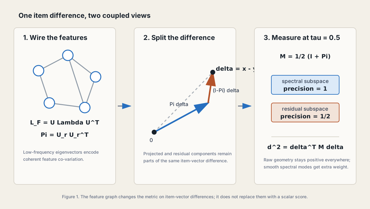
Figure 1 — Wiring the feature graph and its low-frequency projector \(\Pi_F\); splitting an item-vector difference into spectral and residual components; measuring both under the hybrid metric \(\lambda_{0.5}^\tau=\frac12(I+\Pi_F)\).

Feature-manifold projection

Let the symmetric feature Laplacian admit the eigendecomposition

where \(U=[u_1,\ldots,u_F]\) contains feature-space eigenvectors ordered from low to high spectral frequency.

Choose a spectral subspace \(U_{\le r}\) containing the first \(r\) meaningful modes, excluding any trivial constant mode where appropriate. Define the spectral projection

For an item vector \(x\in\mathbb R^F\),

is the component of the item that is smooth and coherent with the wired feature manifold.

The residual,

contains variation that the selected spectral manifold does not explain. Depending on the chosen modes, this residual can represent local novelty, high-frequency structure, noise, or off-manifold behaviour.

ArrowSpace’s feature-first wiring constructs the Laplacian over feature relationships, so applying \(\Pi_F\) to an item vector is precisely an item-space operation conditioned by the feature manifold. ¹³

A 50–50 hybrid distance

For two item vectors \(x,y\in\mathbb R^F\), define the geometric distance

and the spectral-projection distance

With \(\tau=0.5\), define the ArrowSpace spectral-geometric distance

Therefore,

Both terms are norms of differences between item vectors; the second norm is evaluated after a feature-manifold projection.

Distance to the dataset

The spectral-geometric distance from a point \(x\) to the dataset is

The corresponding spectral-geometric projection is

In words, \(\operatorname{proj}^{(0.5)}_{\mathcal K}(x)\) is the training item that is closest to \(x\) after giving equal weight to:

• Raw displacement in the original item geometry.
• Displacement along the projected feature-manifold geometry.

This objective does not require an independent lambda-distance term. The spectral structure is already present in the transformed geometry through \(\Pi_F(x-y)\).

Smoothed hybrid distance

For a finite training set, nearest-point projection is discontinuous at boundaries where more than one item is equally close. As in standard diffusion theory, replace the hard minimum with a soft minimum.

Define the smoothed squared-distance potential

This function has the same role as the ordinary smoothed squared-distance potential, except that nearby points are selected by the feature-manifold-conditioned geometry.

Define the soft assignment weights

The soft spectral-geometric projection is then

At large \(\sigma\), the weights average broad regions of the dataset. At small \(\sigma\), they concentrate around nearby items under the hybrid metric.

Denoising as projection

Differentiating the hybrid potential gives

so the gradient is preconditioned by \(\lambda_{0.5}^\tau\). This is expected: the potential measures displacement in a metric whose geometry depends on the feature-manifold projector.

To recover the actual displacement from the current noisy point to its soft projection, apply the metric correction:

The ideal spectral-geometric denoiser is therefore

Its clean prediction is

So the denoiser performs an approximate projection in the hybrid geometry: it moves toward a weighted mean of data items that are jointly close in raw coordinates and in their spectral projections.

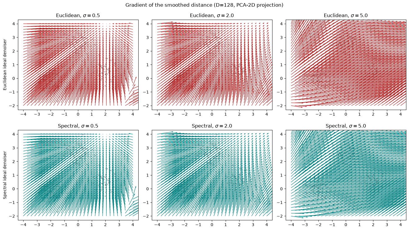
Figure 4 — Gradient of the smoothed squared-distance function on a \(D=128\) multi-cluster dataset (projected to PCA-2D for visualisation). Top row: Euclidean ideal denoiser produces radial fields pointing toward cluster centroids. Bottom row: spectral-geometric ideal denoiser produces elliptical fields aligned with the feature-manifold projector \(\Pi_F\). At \(\sigma=0.5\) both concentrate on nearest neighbours, but the spectral field is already anisotropic; at \(\sigma=5.0\) the Euclidean field averages all clusters uniformly while the spectral field preserves directional structure from the feature graph.

The forward process must match the metric

This is the critical correction. If noise is drawn isotropically — \(x_\sigma = x_0 + \sigma\epsilon\) with \(\epsilon\sim\mathcal N(0,I)\) — then the Bayes-optimal denoiser under any fixed positive-definite reconstruction metric \(M\) is still the conditional mean \(\mathbb E[x_0\mid x_\sigma]\), which is identical to the Euclidean score. Reweighting the loss by \(M\) changes the training emphasis on different directions but does not change the optimal denoiser.

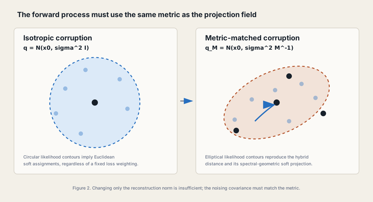
Figure 2 — Left: isotropic corruption produces circular likelihood contours, so soft assignments collapse to Euclidean nearest neighbours regardless of the loss weighting. Right: metric-matched corruption with covariance \(\sigma^2 {\lambda_{0.5}^\tau}^{-1}\) produces elliptical contours aligned with the hybrid geometry, and soft projection naturally follows the spectral-geometric metric.

To make the hybrid distance actually govern the soft assignment, the forward corruption must use the metric’s inverse covariance:

Equivalently, \(x_\sigma\mid x_0 \sim \mathcal N(x_0,\;\sigma^2 {\lambda_{0.5}^\tau}^{-1})\). The likelihood term in the posterior is then

so the soft assignment weights \(w_\sigma\) in Equation (4) arise from the forward process itself, not from an externally imposed distance.

At \(\tau=0.5\), the precision matrix \(\lambda_{0.5}^\tau=\frac12(I+\Pi_F)\) assigns:

• Precision 1 to spectral (low-frequency) directions, where \(\Pi_F\) acts as identity.
• Precision \(\tfrac12\) to residual (high-frequency) directions, where \(\Pi_F\) acts as zero.

This means smooth, coherent feature-manifold variation is corrupted less than off-manifold residual variation. The denoiser learns to be more conservative along spectral directions and more aggressive along residual ones — precisely the asymmetry the hybrid metric encodes.

Training objective

With metric-matched corruption, the standard noise-prediction loss

already targets the hybrid-geometry score, because the model sees inputs whose noise shape is elliptical in \(\lambda_{0.5}^\tau\).

A direct projected reconstruction objective that makes the 50–50 requirement explicit is

where \(\hat x_0 = x_\sigma - \sigma\,\epsilon_\theta(x_\sigma,\sigma)\). Equivalently,

The first half requires fidelity to the observed vector. The second half requires fidelity after projection onto the ArrowSpace feature manifold. The model cannot improve only by matching a spectral scalar; it must predict an item vector whose manifold-projected coordinates are correct.

Training pseudocode

class SpectralGeometry:
    def __init__(self, projector: torch.Tensor, tau: float = 0.5):
        self.Pi = projector
        self.tau = tau
        self.M = tau * torch.eye(projector.shape[0]) + (1.0 - tau) * projector
        self.M_inv_sqrt = self._matrix_inv_sqrt(self.M)

    def project(self, x: torch.Tensor) -> torch.Tensor:
        return x @ self.Pi.T

    def squared_distance(
        self, x: torch.Tensor, y: torch.Tensor
    ) -> torch.Tensor:
        geometric = ((x - y) ** 2).sum(dim=-1)
        spectral = ((self.project(x) - self.project(y)) ** 2).sum(dim=-1)
        return self.tau * geometric + (1.0 - self.tau) * spectral

    def corrupt(
        self, x0: torch.Tensor, sigma: torch.Tensor
    ) -> tuple[torch.Tensor, torch.Tensor]:
        eps = torch.randn_like(x0)
        noise_scale = sigma[:, None] * self.M_inv_sqrt
        x_sigma = x0 + noise_scale * eps
        return x_sigma, eps

    def reconstruction_loss(
        self, x_hat: torch.Tensor, x_true: torch.Tensor
    ) -> torch.Tensor:
        geometric = ((x_hat - x_true) ** 2).mean()
        spectral = (
            (self.project(x_hat) - self.project(x_true)) ** 2
        ).mean()
        return self.tau * geometric + (1.0 - self.tau) * spectral

    @staticmethod
    def _matrix_inv_sqrt(M: torch.Tensor) -> torch.Tensor:
        eigvals, eigvecs = torch.linalg.eigh(M)
        return eigvecs @ torch.diag(1.0 / torch.sqrt(eigvals)) @ eigvecs.T

def training_loop(loader, model, schedule, spectral_geometry, epochs):
    optimizer = torch.optim.Adam(model.parameters())

    for _ in range(epochs):
        for x0 in loader:
            optimizer.zero_grad()

            sigma = schedule.sample_batch(x0)
            x_sigma, eps = spectral_geometry.corrupt(x0, sigma)

            eps_hat = model(x_sigma, sigma)
            x_hat = x_sigma - sigma[:, None] * eps_hat

            loss_noise = ((eps_hat - eps) ** 2).mean()
            loss_projection = spectral_geometry.reconstruction_loss(x_hat, x0)

            loss = 0.5 * loss_noise + 0.5 * loss_projection
            loss.backward()
            optimizer.step()

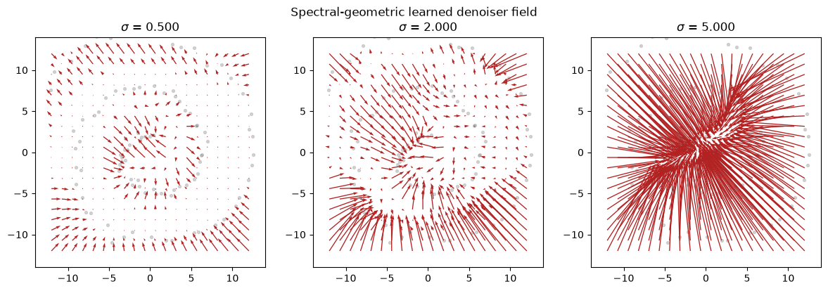
Figure 3 — The spectral-geometric denoiser field on the 2-D Swiss roll (\(\tau=0.5\)). Each arrow points from a noisy point \(x\) to its predicted clean target \(\hat x_0 = x - \sigma \epsilon_\theta(x, \sigma)\). At high \(\sigma\) the denoiser projects toward the spiral centre; at low \(\sigma\) it snaps to the nearest arc segment. The metric-matched corruption ensures the denoiser respects both raw geometry and the feature-manifold projection.

The feature projector must be computed once from the ArrowSpace feature Laplacian and then held fixed during a diffusion run. Recomputing it per noisy minibatch would change the geometry being optimised and destroy the fixed-manifold interpretation. ArrowSpace similarly retains projection metadata so query and indexed vectors are evaluated consistently in the same projected feature space. ³

Hybrid sampling

The deterministic sampling update retains its familiar form:

But its interpretation changes. The update is now an approximate descent step toward the spectral-geometric data manifold:

A sampled trajectory is no longer asked only to approach realistic coordinates. It is asked to approach a point whose coordinate pattern remains coherent after the feature-manifold projection.

@torch.no_grad()
def sample_spectral_geometric(model, sigmas, batch_size):
    x = model.rand_input(batch_size) * sigmas[0]

    for i in range(len(sigmas) - 1):
        sigma = sigmas[i]
        sigma_prev = sigmas[i + 1]
        eps = model(x, sigma.to(x).expand(x.shape[0]))
        x = x - (sigma - sigma_prev) * eps

    return x

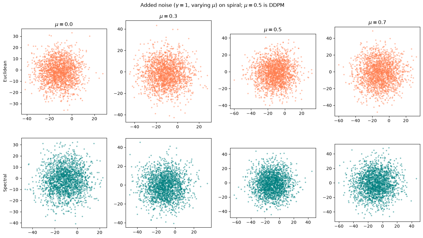
Figure 5 — Sampling with added noise (\(\gamma=1\), varying \(\mu\)) on the spiral manifold in \(D=128\) (PCA-2D projection). Top row: Euclidean diffusion. Bottom row: spectral-geometric diffusion. At \(\mu=0\) (DDIM, deterministic) both produce tight spiral traces. At \(\mu=0.5\) (DDPM) the spectral model preserves the spiral structure better because the metric-matched noise injection respects the feature-manifold directions. At \(\mu=0.7\) both models degrade, but the spectral samples remain closer to the manifold.

No change to the sampler is required if the denoiser has learned the spectral-geometric projection field. The distinction lies in the metric encoded by training and in the fixed ArrowSpace projector supplied to the model or loss.

Interpretation

The standard Euclidean view says that denoising moves a noisy item toward the nearest plausible data vector.

The ArrowSpace view says that denoising moves a noisy item toward a plausible data vector under two equally weighted constraints:

The feature manifold is not an auxiliary retrieval score added after generation. It is a linear geometric operator acting on each item vector before distance is measured. This makes diffusion trajectories sensitive to the structured co-variation of features encoded by the ArrowSpace Laplacian, whose quadratic forms capture spectral smoothness over the wired feature graph. ¹

The key insight this post adds beyond the original adaptation: the forward corruption must share the metric’s covariance structure. Without metric-matched noise (\(\sigma^2 {\lambda_{0.5}^\tau}^{-1}\)), the Bayes-optimal denoiser under any fixed loss weighting collapses to the Euclidean conditional mean. The spectral-geometric structure enters the model only when the noise itself is shaped by the feature manifold.

Implementation notes

• This example use a 50-50 linear combination of geometric and spectral signals but it would be nice to explore potential improvements using different mixes of signals
• Construct \(L_F\) from the training corpus, not from noisy samples generated during diffusion.
• Use a fixed eigenspace cutoff \(r\), selected by spectral gap, explained spectral mass, or validation performance.
• Normalise item vectors and Laplacian conventions consistently before fitting \(\Pi_F\); otherwise the geometric and projected terms will not have comparable scale.
• Keep \(\tau=0.5\) fixed for the stated equal blend. If later made tunable, \(\tau\) should be validated as a geometric metric parameter, not treated merely as a ranking weight.
• Compute \({\lambda_{0.5}^\tau}^{-1/2}\) once and cache it; it is the Cholesky-like factor that maps isotropic Gaussian noise into metric-matched noise.
• Store \(\Pi_F\), \({\lambda_{0.5}^\tau}^{-1/2}\), the eigenspace selection rule, Laplacian configuration, and preprocessing transforms with the diffusion checkpoint. ArrowSpace’s build pipeline likewise preserves projection-related state to ensure consistent query-time computation. ³

ArrowSpace: pip install arrowspace
Rust source: arrowspace-rs
ArrowSpace paper: JOSS — Spectral Indexing of Embeddings
Previous post: ArrowSpace for Latent Spaces — part 2