ArrowSpace for Latent Spaces — part 2
Comparative Semantic Probing: Token Space vs Weight Space
This is the second post in the series on applying ArrowSpace to mechanistic analysis of latent spaces. Part 1 established that ArrowSpace’s Rayleigh energy provides independent, complementary structure to item-space methods for finding local minima. This post goes deeper: instead of probing the output embedding manifold, we probe the transformer weight matrices themselves — treating each layer’s Q/K/V/O/FFN matrices as spectral operators that encode semantic fields in their geometry.
Notebook: 06_B_comparative_semantic_probing.ipynb
Model: all-MiniLM-L6-v2 (6-layer MiniLM-BERT, 384-dim residual stream)
Two Probes, Two Questions
The notebook defines two complementary probing strategies against the same 80-word corpus spanning four semantic fields (FOOD, SCIENCE, TOOL, COLOUR).
Probe A — Token Space (\(E_\text{tok}\)): Extract the raw static embedding for each word via a direct lookup in the token embedding matrix:
\[E_\text{tok}[\text{token_id}] \in \mathbb{R}^{384}\]This vector is the pre-attention token direction — the signal the model receives before any attention or FFN layer has processed it. Projecting it through a weight matrix \(W\) answers a direct circuit-level question: how does this layer transform a raw input signal?
Probe B — Weight Space (model.encode): Run the full 6-layer transformer and extract the mean-pooled contextualised embedding:
This encodes how the model contextualises the word given its pre-training. But projecting it back through, say, \(W_q\) at layer 3 introduces a self-consistency bias: that very matrix partially shaped \(X_\text{pass}\) during the forward pass. The notebook explicitly quantifies this inflation at 7–16% extra activation energy across fields, and treats it as a documented epistemic limit rather than a correction. This is a self-evident as it is how the model is supposed to work, so Probe B it is just a confirmation that the probing in spotting some difference (B minus A below).
The two probes are designed to be contrasted: where they diverge, the transformer has performed non-trivial re-encoding; where they agree, the raw token geometry is largely preserved.
| Aspect | Probe A: \(E_\text{tok}\) | Probe B: model.encode |
|---|---|---|
| Represents | Pre-attention token direction | Contextualised semantic embedding |
| Bias | None — clean circuit-level input | Self-consistency (7–16% inflation) |
| What it measures | How weights transform a raw signal | How weights recognise their own output |
| Single-token guarantee | ✅ One word → one \(E_\text{tok}\) row | ❌ Full attention over BOS/EOS tokens |
| Mechanistic value | More tractable; direct circuit analysis | More downstream; emergent representation |
Why single-token words? The corpus is restricted to words that tokenise to exactly one subword ID, enforcing a 1-to-1 mapping from word to \(E_\text{tok}\) row. This eliminates subword averaging artefacts and makes Probe A a clean circuit-level test.
The Activation Energy as a Rayleigh Analogue
For every combination of layer index \(i\) and weight role \(r\), the notebook computes a Frobenius-normalised projection norm:
\[E(W, x) = \frac{\|W\, x\|_2}{\|W\|_F + \varepsilon}\]This is a linear analogue of ArrowSpace’s Rayleigh quotient:
\[R(x) = \frac{x^\top L\, x}{x^\top x} \quad \xrightarrow{\text{ArrowSpace}} \quad \lambda_w(x) = w \cdot R_\text{geom}(x) + (1-w) \cdot R_\text{spec}(x)\]where \(L\) is the normalised graph Laplacian built from the kNN feature graph. The analogy holds at two levels:
| ArrowSpace \(\lambda\) | Weight-space probe \(E\) |
|---|---|
| \(L = \Phi\,\Lambda\,\Phi^\top\) — Laplacian of the data graph | \(W\) — a single transformer weight matrix |
| \(R(x) = x^\top L\, x / |x|^2\) — energy on the data manifold | \(E(W,x) = |Wx|_2 / |W|_F\) — energy in the weight subspace |
| Low \(\lambda\) → smooth, dense semantic basin | Low \(E\) → weakly activated by that matrix |
| High \(\lambda\) → spectral boundary or anomaly | High \(E\) → strongly excites the weight direction |
The key difference: \(R(x)\) is built from dataset topology (how items relate via the kNN graph). \(E(W, x)\) is built from model topology (how a frozen weight matrix responds to a token direction).
The Dual-Space Decomposition
Dual space is a fundamental characteristics of ArrowSpace/Graph Wiring, every vector space is leveraged by its geometric space (item-space) and its semantic space (feature-space). The contribution of feature-space has been demonstrated to be relevant as measured by epiplexity in this paper and the source of the advanteages provided in search capabilities.
The notebook introduces a conceptually important split in how the two FFN matrices are treated. Each of the 6 transformer layers contains:
-
\(W_\text{ffn1}\) (primal / write operator): shape
(1536, 384)— projects the 384-dim residual stream up into the 1536-dim FFN hidden space. Used as a standard projection: \(\|W_\text{ffn1}\, x\|_2 / \|W_\text{ffn1}\|_F\). -
\(W_\text{ffn2_read}\) (dual / readout operator): the FFN output matrix has shape
(384, 1536). For probing, its transpose is used — shape(1536, 384)— measuring \(\|W_\text{ffn2}^\top x\|_2 / \|W_\text{ffn2}\|_F\). This answers: which FFN hidden neurons are most sensitive to this token direction?
This mirrors ArrowSpace’s own primal/dual split. In ArrowSpace the item-space Laplacian operates on \(X\) (items × features), while the feature-space Laplacian operates on \(X^\top\) (features × items). Treating \(W_\text{ffn1}\) as a write operator and \(W_\text{ffn2}^\top\) as a readout operator is precisely the same structural inversion — applied to transformer circuits rather than embedding graphs.
The extracted layer structure is:
Extracted 36 weight matrices across 6 layers.
  Layer 0 | W_q     → shape (384, 384)
  Layer 0 | W_k     → shape (384, 384)
  Layer 0 | W_v     → shape (384, 384)
  Layer 0 | W_o     → shape (384, 384)
  Layer 0 | W_ffn1  → shape (1536, 384)
  Layer 0 | W_ffn2  → shape (384, 1536)
Each layer contributes six subspaces: four attention roles (Q/K/V/O), one primal FFN write (W_ffn1), and one dual FFN readout (W_ffn2_read via transpose). Across 6 layers that is 36 weight-role subspaces probed per word.
Semantic Subspace Matrices
For each of the 36 (layer × role) subspaces and each of the 4 semantic fields, the notebook computes a normalised contrast score:
\[S_{(i,r,f)} = \frac{\bar{A}_{(i,r,f)} - \bar{A}_{(i,r,\neg f)}}{\bar{A}_{(i,r,f)} + \bar{A}_{(i,r,\neg f)} + \varepsilon} \in [-1, +1]\]A filled dot in the scatter diagram marks the dominant field in that subspace; hollow dots mark secondary presence.
Fig 03a — Probe A: raw \(E_\text{tok}\) space
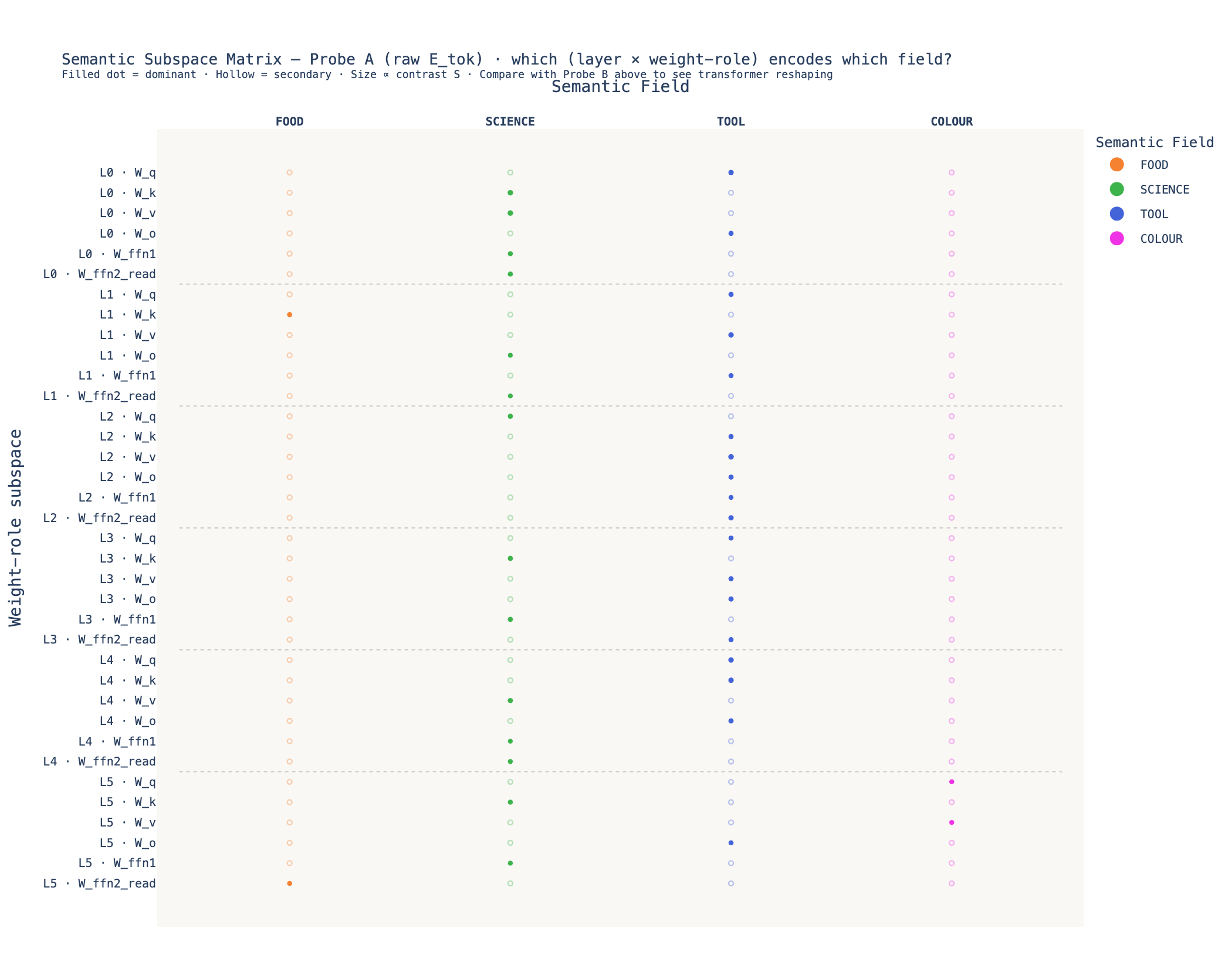
Probe A reveals the raw token geometry as seen by each weight matrix. SCIENCE and TOOL dominate across layers 0–4. COLOUR only surfaces in layer 5 (W_q, W_v) — it is spectrally flat in the raw token space, becoming decodable only after the model has processed the sequence.
The dominant-field table for Probe A (excerpt):
| Subspace | Dominant Field | Contrast S | Top Words |
|---|---|---|---|
| L0 · W_q | TOOL | 0.017 | wheel, forge, knife |
| L0 · W_k | SCIENCE | 0.019 | protein, energy, gene |
| L0 · W_v | SCIENCE | 0.023 | photon, energy, protein |
| L0 · W_ffn1 | SCIENCE | 0.012 | circuit, enzyme, neutron |
| L0 · W_ffn2_read | SCIENCE | 0.011 | enzyme, virus, neutron |
| L2 · W_ffn2_read | TOOL | 0.016 | drill, drill, vice |
| L5 · W_q | COLOUR | 0.007 | purple, orange, crimson |
| L5 · W_ffn2_read | FOOD | 0.011 | tea, milk, rice |
Fig 03b — Probe B: full transformer pass
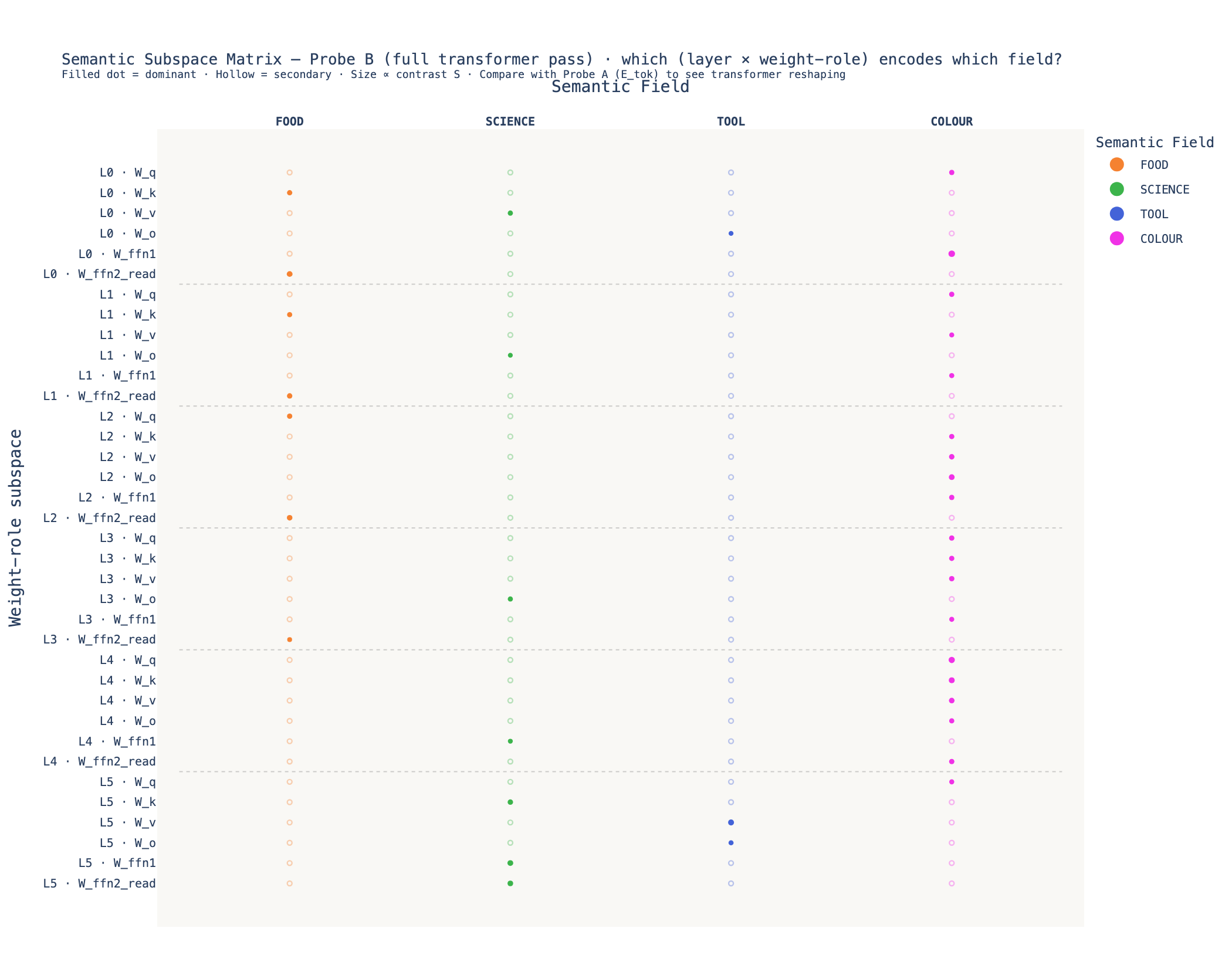
After the full transformer pass, the pattern shifts. FOOD gains strong dominance in the W_ffn2_read dual subspaces at layers 0–2 (contrast up to S = 0.029), SCIENCE consolidates at layer 5 (W_ffn1 S = 0.029, W_ffn2_read S = 0.026). The dual readout subspaces show the largest absolute contrast scores in both probes — the FFN transpose is the most field-selective axis in the model.
The Probe A/B per-field energy delta (primal roles):
| Field | Mean E (Probe A) | Mean E (Probe B) | Δ% |
|---|---|---|---|
| COLOUR | 0.04695 | 0.05277 | +12.4% |
| FOOD | 0.04679 | 0.05197 | +11.1% |
| SCIENCE | 0.04780 | 0.05214 | +9.1% |
| TOOL | 0.04782 | 0.05127 | +7.2% |
The dual/readout delta is consistently larger than the primal delta (FOOD +15.8%, TOOL +14.1%). This is consistent with the self-consistency bias hypothesis: the FFN readout neurons recognise their own outputs more strongly than the attention write operators do.
Fig 03c — \(\Delta S\) Dual Space
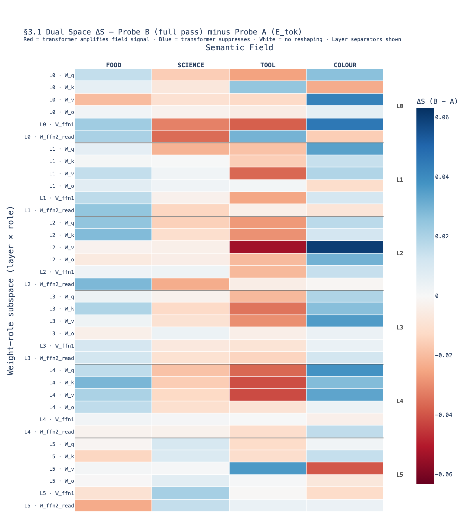
The \(\Delta S\) figure shows the difference in contrast score between Probe B and Probe A for the dual (W_ffn2_read) subspaces only. Positive values indicate fields where full transformer contextualisation adds discriminative power beyond raw token geometry. FOOD and SCIENCE show the largest positive \(\Delta S\) in the final layer’s dual subspace — meaning the FFN readout at layer 5 is where contextual semantic sharpening is most visible.
What the Three Figures Show Together
The trio of figures maps a single question — where does semantic field structure live in the weight geometry? — across three views:
-
Fig 03a (Probe A): The raw token space already contains substantial SCIENCE/TOOL signal in layers 0–4. The weight matrices do not start from a blank slate; the token embedding matrix carries pre-trained semantic structure that the attention layers then redistribute.
-
Fig 03b (Probe B): The full transformer sharpens field separation, particularly in the dual/readout subspaces and at the final layer. FOOD rises in the FFN readout at layers 0–2; SCIENCE and COLOUR sharpen at layer 5. The last layer’s dual subspace (
L5 · W_ffn2_read) carries the strongest context-dependent signal. -
Fig 03c (\(\Delta S\) dual): The difference reveals where the transformer performs meaningful re-encoding. The final FFN readout is the primary site of contextual semantic amplification — a mechanistic anchor for the ArrowSpace spectral lens.
The Principled Dual-Space Anchor
The strongest result in this notebook is not a single number but a structural correspondence. The primal/dual split — \(W_\text{ffn1}\) as a write operator, \(W_\text{ffn2}^\top\) as a readout operator — directly mirrors ArrowSpace’s own feature-space Laplacian:
\[L_\text{feat} = X X^\top \quad \text{(item-space)} \quad \longleftrightarrow \quad L_\text{item} = X^\top X \quad \text{(feature-space)}\]This is not an empirical heuristic imposed after the fact. The FFN architecture is literally a write-then-read structure in higher-dimensional space, and treating \(W_\text{ffn2}^\top\) as the readout axis is the mechanistically correct interpretation. ArrowSpace’s spectral language — Rayleigh quotients, Laplacian smoothness, primal/dual Laplacians — provides a single framework that spans all three objects: the semantic embedding graph, the feature-space graph, and the transformer weight circuits.
The bias-awareness is also worth noting cleanly: Probe B’s self-consistency inflation (7–16%) is documented in the notebook’s code comments, not buried. If you use model.encode activations to probe the same weight matrices that shaped them, you get inflated scores — and this notebook tells you by exactly how much per field.
Scale-Up Paths
The methodological bridge from this 80-word BERT experiment to production-scale LLMs is direct. The activation energy \(E(W, x)\) scales linearly in the number of weight matrices, independent of ambient dimension. For a model like LLaMA-3 70B (~1,000 weight matrices), batching across GPUs produces a \(\lambda\)-indexed circuit map: which (layer, role) pairs fire for which semantic fields under the ArrowSpace spectral vocabulary.
Four concrete directions follow from the dual-space decomposition:
-
Layer-wise activation manifold indexing. Build one ArrowSpace index per layer from residual stream activations on a domain corpus. The \(\lambda\)-score becomes a layer-resolved semantic energy surface — identifying dense basins (low \(\lambda_\text{full}\)) vs boundary tokens (high \(\lambda_\text{spec}\)) analogous to the layer-by-layer heatmaps here.
-
Weight-space circuit localisation. The primal/dual heatmap (4 fields × 6 layers) expands to a semantic-field × layer grid for any target vocabulary. The dual readout axis (\(W_\text{ffn2}^\top\)) is the most field-selective probe and should be the first target for circuit-level ablations.
-
Latent space basin monitoring. A persistent ArrowSpace index over inference activations flags tokens drifting into high-\(\lambda_\text{spec}\) regions — spectral boundaries of the trained manifold. This is strictly richer than cosine-based drift detection because it captures graph connectivity, not only pairwise distance.
-
\(\lambda\)-indexed circuit ablation. Tokens at spectral boundaries (high \(R_\text{spec}\)) before ablation are candidates for “transition zones” in the circuit — the exact locations where activation patching has the largest causal effect. The \(\lambda\)-score provides a cheap, geometry-grounded prior for prioritising ablation targets, reducing the combinatorial search space without any model modifications.
Conclusion
We have presented here the first simple example of Graph Wiring used as a mechanistic interpretability primitive, treating transformer weight matrices as spectral operators on a semantic kNN graph so that ArrowSpace’s Rayleigh-style energy cleanly links embedding geometry, Laplacian smoothness, and layer-wise circuit probes under one unified spectral language.
Graph wiring — the kNN topology that ArrowSpace draws on the feature manifold — here becomes a mechanistic interpretability primitive: a Frobenius-normalised projection norm that maps which weight-matrix subspaces encode which semantic fields, layer by layer, in both the primal write direction and its dual readout transpose.
- Graph Wiring: Eigenstructures for vector datasets and LLM operations
- Epiplexity And Graph Wiring: An Empirical Study for the Design of a Generic Algorithm
- Spectral Indexing using taumode (λτ) with arrowspace
- ArrowSpace: Spectral Search For Embeddings and Graph Analysis
Notebook: 06_B_comparative_semantic_probing.ipynb
Figures: fig_03a, fig_03b, fig_03c
Previous post: ArrowSpace for Latent Spaces — part 1
ArrowSpace: pip install arrowspace