Condense, Project, and Sparsify
You can find arrowspace in the:
- Rust repository ↪️
cargo add arrowspace - and Python repository ↪️
pip install arrowspace
Road for arrowspace to scale: this release v0.13.3 rethinks how arrowspace builds and queries graph structure from high‑dimensional embedding up to 10⁵ items and 10³ features. The Laplacian computation now:
1) condenses data with clustering and density‑aware sampling,
2) projects dimensionality proportionally to the problem size (centroids) and keeps queries consistent with that projection, and
3) sparsifies the graph with a fast spectral method to preserve structure while slashing cost.
1) Condense the data first: clustering + density‑adaptive sampling
Building a Laplacian directly on millions of items and thousands of features is expensive; most structure can be captured by a compact set of representatives.
- Clustering to ease Laplacian compute
- Cluster items in embedding space and use the centroids as graph nodes to cut N down by orders of magnitude.
- The Laplacian is then computed over centroids, not raw items, which reduces k‑NN cost, Laplacian storage, and downstream spectral ops.
DensityAdaptiveSamplerfor centroids- Complement or replace clustering with a density‑aware sampler that selects more centroids where the manifold is dense and fewer where it is sparse.
- This keeps neighborhood fidelity without inflating node count, making the resulting k‑NN graph more uniform and robust to hubness/anisotropy.
Practical notes:
- Choose target centroid count from budget, not from original feature count.
- Keep k in the k‑NN graph large enough to avoid fragmentation on the reduced set (e.g., 10–30 for a few hundred centroids).
- Cache centroid assignments if later stages (evaluation, attribution) need to lift results back to original items.
- This is practically equivalent to IVF, so it is possible to go a step further to implement IVF-PQ search.
2) Dimensionality Reduction: project to the problem size
After condensing to C centroids, distance preservation only needs to hold between those C points; the Johnson–Lindenstrauss (JL) lemma gives a principled target for the projected dimension r.
- Dimensionality reduction through projection
- Compute r from the number of centroids (not original items), e.g.,
r ≈ 8·ln(C)/ε²for tolerance ε. - Project both centroids and their associated item representations to r dimensions before graph building.
- This reduces memory, improves k‑NN construction time, and helps combat distance concentration in very high dimensions.
- Compute r from the number of centroids (not original items), e.g.,
- Querying with projection
- At query time, apply the same projection (same random seed / matrix) to the incoming vector, then compute the synthetic λ on the projected graph and search in the projected space.
- This keeps train/test geometry aligned: the Laplacian, λ synthesis, and similarity all “see” the same r‑dimensional manifold.
Practical notes:
- Normalize features before projection; keep the projection operator fixed per model version (normalise after clustering).
- Pick ε by latency/quality trade‑off; smaller ε → larger r → better geometric fidelity.
- Store r and projection seed with the built artifact so clients can reproject queries deterministically.
3) Make graphs lighter: SF‑GRASS spectral sparsification
Even after condensing and projecting, dense graphs and Laplacians can still be costly. A simplified, fast spectral sparsification (SF‑GRASS) step prunes edges while approximately preserving the spectrum that matters for diffusion, λ computation, and spectral similarity.
- Sparsification (SF‑GRASS)
- Start from the k‑NN (or locally scaled) weighted graph on centroids.
- Apply simplified spectral sparsification to obtain a much sparser graph that preserves quadratic forms xᵀLx within a small relative error.
- This yields a Laplacian that is dramatically cheaper to store and multiply while retaining the eigenstructure relevant to λ and search.
- Storage and ops
- Keep the Laplacian in a sparse format (e.g., CSR/CSC) for all downstream computations.
- Traversals and updates use index pointers instead of dense indexing; eigen or diffusion routines get a sizable acceleration on typical sizes.
Practical notes:
- Target an average degree that keeps the graph connected but trims long, low‑weight tails (e.g., density ~5–20% depending on C and k).
- If local scaling or mutual k‑NN was used pre‑sparsification, sparsification tends to preserve cluster‑local edges especially well.
- Validate PSD and symmetry after sparsification; diagonals remain non‑negative and the smallest eigenvalue stays near zero.
Usage at a glance
- Build:
- Sample or cluster to centroids (C).
- Compute r from C via JL, project items/centroids to r.
- Build a k‑NN (optionally locally scaled) graph over centroids.
- Apply SF‑GRASS to sparsify; store sparse Laplacian and projection.
- Query:
- Project the query to r with the stored projection.
- Compute synthetic λ on the projected Laplacian.
- Search in the projected space with the λ‑aware scorer.
Migration guide
- If code relied on raw items for Laplacian, switch to centroids via clustering or
DensityAdaptiveSampler; propagate centroid mapping where needed. - Introduce a persisted projection (r, seed) tied to the graph artifact; apply it consistently during build and query.
- After building the k‑NN graph, run SF‑GRASS and ensure all Laplacian consumers accept sparse inputs; update tests to iterate via CSR pointers.
- For search, replace ad‑hoc λ heuristics with the unified query path: project → synthesize λ → λ‑aware scoring.
Why this works well together
- Condensing shrinks the node set to what matters; JL then shrinks dimensions to what the node set needs (not what the raw features had); sparsification shrinks edges to what the spectrum needs. The query path mirrors the training path by reusing the same projection and Laplacian, keeping semantics aligned and stable.
New Metrics
Here the new metrics for these improvements, let’s have a reference about what they display. These are all partial and indicative of trends are they are computed on a limited dataset (NxF: 3000x384) of synthetic data.
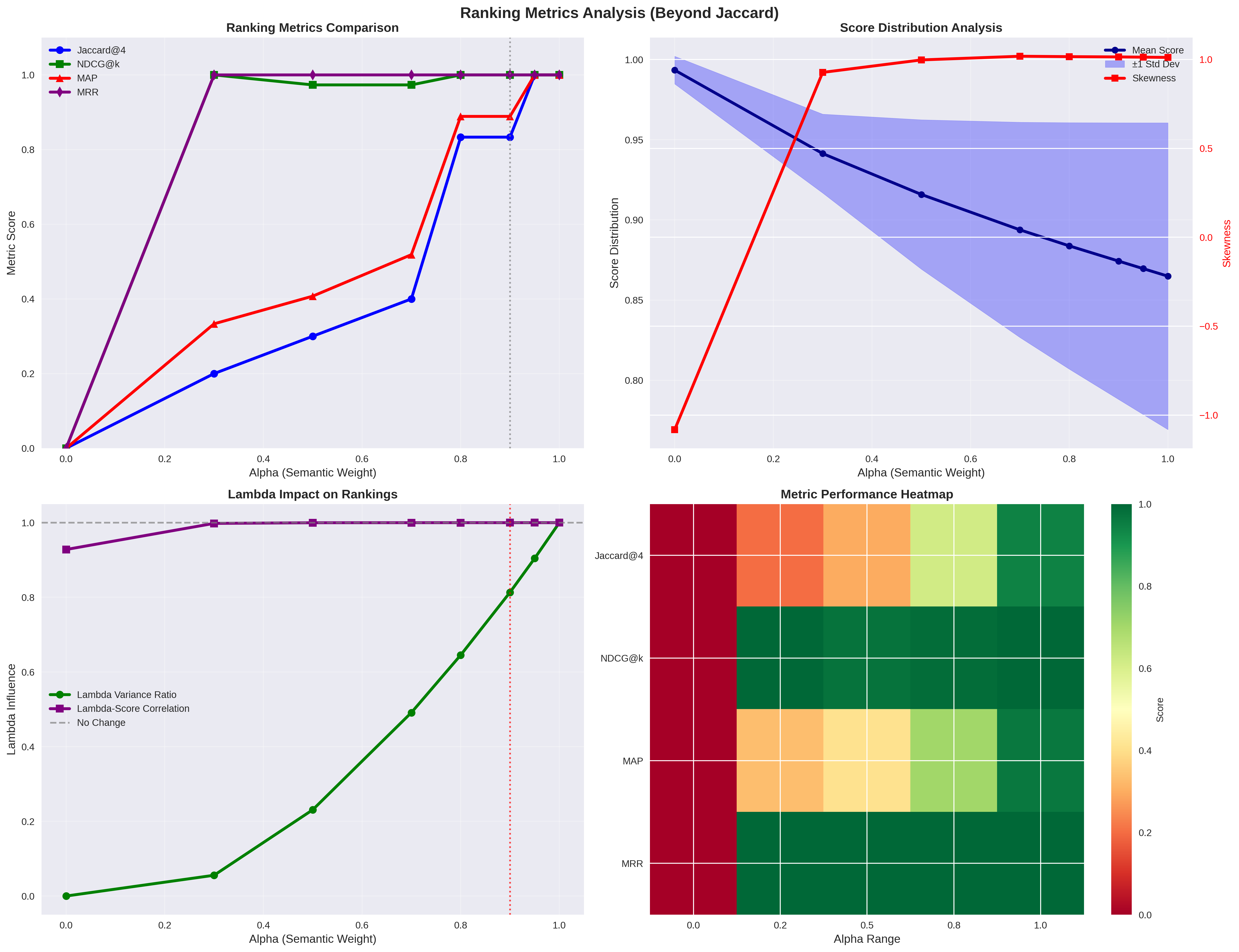
top-left: Ranking Metrics
As one of the main objective of arrowspace is to spot alternative pathways for vector similarities, I use different metrics to compare the new measurements to current implementations. Jaccard metric is quite limited for this purpose as it just spots the perfect overlapping between cosine similarities and arrowspace similarities; for widening the landscape I have introduced in the visualisation NDCG, MAP and MRR. You can see how they compare on the usual scale from alpha=0.0 to alpha=1.0 (the weigth of cosine similarity in the taumode computation). What I read in this is that taumode is still equivalent to cosine similarity between alpha=0.6 and alpha=0.8 while making results more interesting as tails may contain alternative pathways.
A bried summary here for you about these metrics:
- NDCG: Evaluates the quality of ranking by considering both relevance scores and position, with logarithmic discounting for lower positions.
- MAP: Average precision across multiple queries, heavily emphasizing precision at each relevant item position.
- MRR: The average reciprocal of the rank of the first relevant item across queries (less relevant as it focuses only on the first ranked item).
A matrix about the characteristics of these metrics:
| Feature | NDCG | MAP | MRR |
|---|---|---|---|
| Relevance Type | Binary or graded | Binary only | Binary only |
| Scope | Full ranked list | All relevant items | First relevant only |
| Discount | Logarithmic | Precision-based | None (single position) |
| Interpretability | Low (complex formula) | Medium (area under PR curve) | High (average rank) |
| Use Case | Multi-item recommendations | Top-K search results | Single-answer search |
| Sensitivity | Balanced across ranks | Top-heavy | First position only |
bottom-right: Metric Performance Heatmap
I leave the reading of the other two to you. The bottom-right diagram is interesting as it displays how taumode starts to be reliable from alpha=0.6 on all the metrics used.
Next steps include but they are not limited to:
- improve pre-laplacian input data via graph decomposition into sub-graphs
- take some time to finally investigate how to make the queries multi-vector instead of single-vector
- move the basic flow to GPU! So I have to restart from the non-optimised version to build up a GPU-dedicated computation
- Build the database stack for this engine! From the storage layer to the API
Interested in learning more? Whether you’re evaluating ArrowSpace for your data infrastructure, considering sponsorship, or want to discuss integration strategies, please check the Contact page.
Please consider sponsoring my research and improve your company’s understanding of LLMs and vector databases.
Book a call on Calendly to discuss how ArrowSpace can accelerate discovery in your analysis and storage workflows, or discussing these improvements.